QC for Genomics

• Prerequisites

  ---

  • Access to an RCAC cluster (Negishi or Gautschi)
  • Familiarity with the Linux command line (cd, ls, mkdir)
  • A terminal session via Open OnDemand or SSH

• Objectives

  ---

  • Understand why quality control matters at every stage of genomics analysis
  • Run and interpret FastQC reports for raw sequencing reads
  • Aggregate QC results across samples with MultiQC
  • Trim and filter reads with fastp
  • Know what QC metrics to check after alignment and variant calling

Why QC Matters

Quality control is the most important step you can take before starting any genomics analysis. The principle is simple: garbage in, garbage out. If your raw sequencing data has problems such as adapter contamination, low-quality bases, or reads from the wrong organism, every downstream result is compromised. The worst part is that these problems often propagate silently. Your pipeline will still produce output files. You will still get variant calls, expression counts, or an assembly. They will just be wrong.

QC is not a one-time checkbox at the beginning of your workflow. You should check quality at every stage:

• Raw reads: Are the sequences high quality? Is there adapter contamination?
• After trimming: Did trimming improve quality without losing too much data?
• After alignment: What fraction of reads mapped? Are there too many duplicates?
• After variant calling: Are the variant statistics consistent with expectations?
• After assembly: Is the assembly complete? Are there missing genes?

The cost of skipping QC is real: wasted compute hours processing bad data, false positive results that don't replicate, and in the worst case, retracted papers. The good news is that QC is fast and easy. Fifteen minutes of checking quality can save you weeks of troubleshooting.

Setup

Accessing the Cluster

Open OnDemandSSHThinLinc

Recommended starting point. Open OnDemand provides a web portal with a file browser, terminal, job submission forms, and interactive apps like JupyterLab and RStudio. No software to install.

1. Navigate to the OOD portal

   Go to https://gateway.<cluster>.rcac.purdue.edu and log in with your Purdue (BoilerKey) credentials.

   Cluster	OOD URL
   Gautschi	gateway.gautschi.rcac.purdue.edu
   Negishi	gateway.negishi.rcac.purdue.edu
   Bell	gateway.bell.rcac.purdue.edu
   Gilbreth	gateway.gilbreth.rcac.purdue.edu

2. Tour the dashboard

   After login you will see the OOD dashboard with these key sections:

   • Files: Browse, upload, download, and edit files on the cluster
   • Jobs: View active jobs or use the Job Composer to build submission scripts
   • Clusters: Open a shell terminal (equivalent to SSH) directly in the browser
   • Interactive Apps: Launch JupyterLab, RStudio Server, and other GUI applications

3. Open a terminal

   Click Clusters in the top menu and select the cluster shell access (e.g., Gautschi Shell Access). A terminal opens in your browser. You are now on a login node.

Tip

OOD is the fastest way to get started because there are no SSH keys to configure. If you are new to HPC, start here.

SSH gives you direct terminal access. It is built into macOS and Linux. On Windows, use PowerShell, WSL, PuTTY, or MobaXterm.

ssh <boilerid>@gautschi.rcac.purdue.edu

Replace <boilerid> with your Purdue career account username. For other clusters, replace gautschi with the cluster name.

Tip

For password-less login and SSH shortcuts (e.g., ssh gautschi instead of the full hostname), see the SSH Keys and Configuration section of the Productivity Toolkit.

ThinLinc provides a full Linux desktop environment, ideal for GUI-based tools like IGV, CellProfiler, MEGA, or any application that needs a graphical interface.

1. Install the ThinLinc client

   Download and install the ThinLinc client for your operating system from the ThinLinc download page.

2. Connect to the cluster

   Open the ThinLinc client and enter the connection details:

   Field	Value
   Server	desktop.<cluster>.rcac.purdue.edu
   Username	Your Purdue career account (BoilerID)
   Password	Your Purdue password

   For example, to connect to Gautschi: desktop.gautschi.rcac.purdue.edu

3. Authenticate

   After entering your credentials, you will be prompted for Duo two-factor authentication. Approve the push notification or enter the code.

4. Use the desktop

   You now have a full Linux desktop. Open a terminal from the Applications menu to run commands, or launch GUI applications directly.

You can also access ThinLinc through a web browser (no client install needed) at https://desktop.<cluster>.rcac.purdue.edu/. The native client generally provides a smoother experience.

For detailed ThinLinc documentation, see the RCAC ThinLinc guide.

Set Up Your Working Directory

cd $RCAC_SCRATCH
mkdir -p genomics_exchange/session6
cd genomics_exchange/session6

Load Modules

RCAC provides bioinformatics software through the module system. Always start with a clean environment:

module --force purge

We will load specific tool modules as needed in each section below.

FastQC: Assessing Raw Read Quality

FastQC is the standard tool for assessing the quality of sequencing data. It takes FASTQ files as input and produces an HTML report with visualizations of key quality metrics.

Understanding FASTQ Format

Before running FastQC, it helps to understand what a FASTQ file looks like. Each read in a FASTQ file consists of four lines:

@read_name             <- Read identifier
ACGTACGTACGT...        <- DNA sequence
+                      <- Separator
IIIIIHHHGG...          <- Quality scores (one character per base)

The quality scores on line 4 are encoded as ASCII characters. Each character represents a Phred quality score: a measure of how confident the sequencer is that it read each base correctly.

Phred Score	Error Probability	Accuracy
Q10	1 in 10	90%
Q20	1 in 100	99%
Q30	1 in 1,000	99.9%
Q40	1 in 10,000	99.99%

Modern Illumina sequencers typically produce data with Q30 or higher for most bases. Q20 is generally considered the minimum acceptable quality.

What is Paired-End Sequencing?

In paired-end sequencing, both ends of each DNA fragment are read, producing two files per sample: R1 (forward read) and R2 (reverse read). This gives you more information about where each fragment came from in the genome and is the most common approach for Illumina sequencing.

Running FastQC

1. Load the FastQC module:

   module load biocontainers fastqc/0.12.1
   

2. Create an output directory and run FastQC:

   mkdir -p fastqc_raw
   fastqc -t 4 -o fastqc_raw/ raw_reads/sample1_R1.fastq.gz raw_reads/sample1_R2.fastq.gz
   

   • -t 4: use 4 threads (one per file, speeds things up)
   • -o fastqc_raw/: write output to this directory

3. For multiple samples, loop over all files:

   for fq in raw_reads/*.fastq.gz; do
       fastqc -t 4 -o fastqc_raw/ "$fq"
   done
   

4. View the HTML report. You can open it through the Open OnDemand file browser (navigate to the file and click on it) or download it to your laptop:

   scp boilerid@negishi.rcac.purdue.edu:$RCAC_SCRATCH/genomics_exchange/session6/fastqc_raw/sample1_R1_fastqc.html .
   

Interpreting FastQC Modules

FastQC evaluates 12 quality modules. Each module gets a pass (green check), warn (orange triangle), or fail (red X) status. The table below explains what each module measures and how to interpret it.

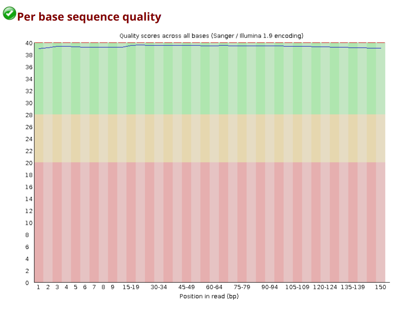
A healthy per-base quality plot looks like this: scores stay in the green zone (Q28+) across the entire read, with only a small dip at the 3' end.

Module	What It Measures	Good	Bad	Common False Flags
Basic Statistics	Read count, length, GC%	Consistent with expectations	Unexpected read count or length	Rarely triggers false flags
Per Base Sequence Quality	Phred scores at each position along the read	Q28+ across most positions; slight drop at 3' end is normal	Q < 20 across large portions of the read	Rarely false; always investigate
Per Tile Sequence Quality	Quality variation across flow cell tiles	Uniform blue heatmap	Hot spots (yellow/red patches) indicate flow cell problems	Rare
Per Sequence Quality Scores	Distribution of average quality per read	Single peak at Q30-Q37	Bimodal distribution (two peaks)	Rare
Per Base Sequence Content	%A, %T, %G, %C at each position	Roughly equal A/T and G/C; flat lines	Strong bias throughout the read	First 10-15 bases often wobble due to random hexamer priming. This is normal
Per Sequence GC Content	Distribution of GC% across all reads	Smooth bell curve matching your organism	Bimodal curve = contamination from another organism	Rarely false; investigate if unexpected
Per Base N Content	Percentage of N (unknown) bases at each position	Near 0% everywhere	Spikes of N calls indicate sequencer problems	Rare
Sequence Length Distribution	Distribution of read lengths	All reads same length (pre-trimming)	Unexpected variation	After trimming, variation is expected and normal
Sequence Duplication Levels	How many reads appear more than once	Most reads unique (low duplication)	High duplication in WGS = low library complexity	RNA-seq: high duplication is normal (highly expressed genes). Amplicon: high duplication is expected.
Overrepresented Sequences	Sequences making up > 0.1% of reads	None or very few	Adapter sequences, rRNA contamination	RNA-seq: abundant transcripts trigger this. Not always a problem.
Adapter Content	Cumulative adapter contamination at each position	Near 0% throughout	Rising curves at read ends = adapter read-through	Rarely false; needs trimming if present
Kmer Content	Overrepresented short sequences at specific positions	No enrichment	Enrichment at specific positions = primer or adapter contamination	First few bases often enriched due to priming bias, usually normal

Warning

FastQC's pass/warn/fail flags are calibrated for whole-genome shotgun (WGS) data. If you are working with RNA-seq, amplicon, bisulfite, or other specialized data types, expect false warnings on several modules. The flags are a starting point, not a verdict; you must interpret them in context.

Visual Reference: Good vs Problematic Patterns

The cartoons below (by Zandra Selina, CC BY 4.0) show what each module looks like for healthy data and for the most common failure modes. Use them as a quick mental lookup when you open a real report.

Per Base Sequence Quality (R1 vs R2)

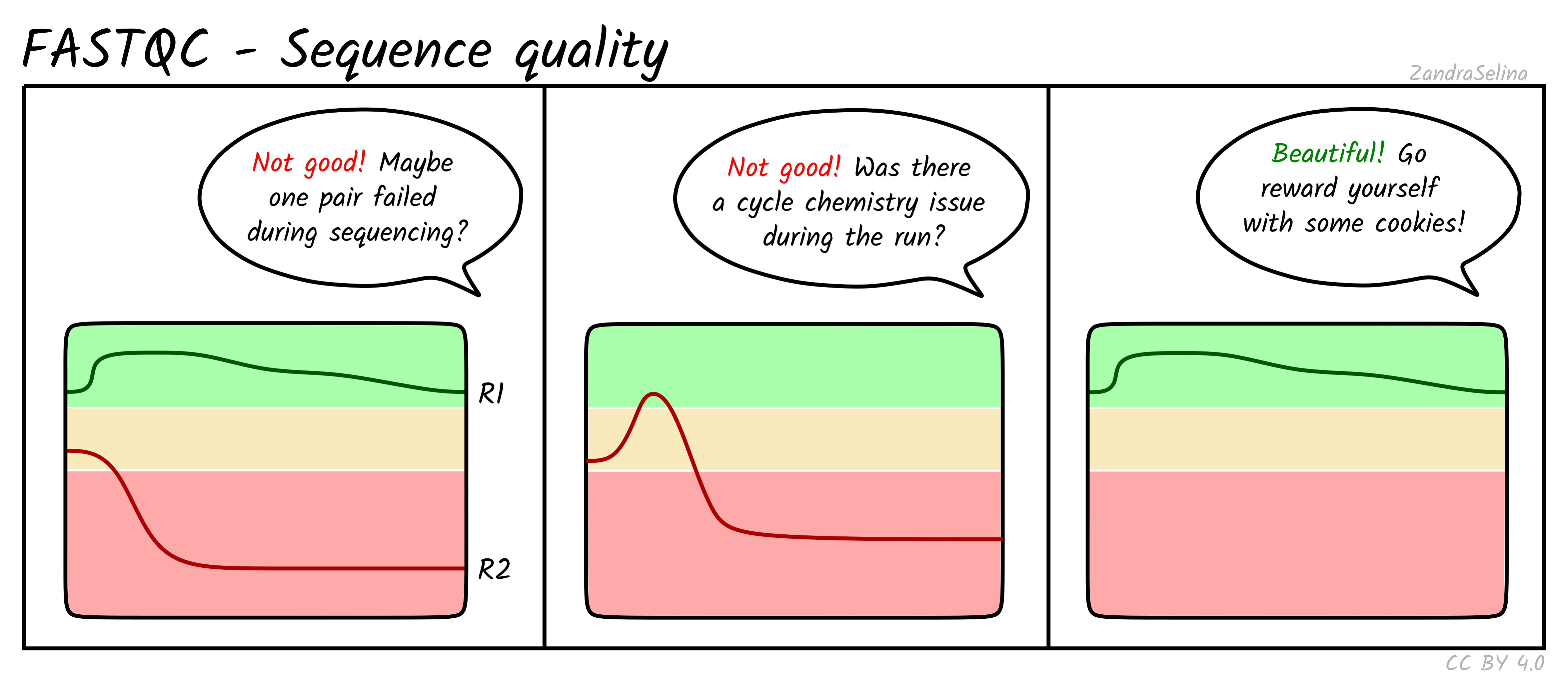
R2 is expected to be slightly worse than R1, but a sharp collapse or a mid-read dip points to a sequencing run problem rather than a library issue.

Per Sequence GC Content

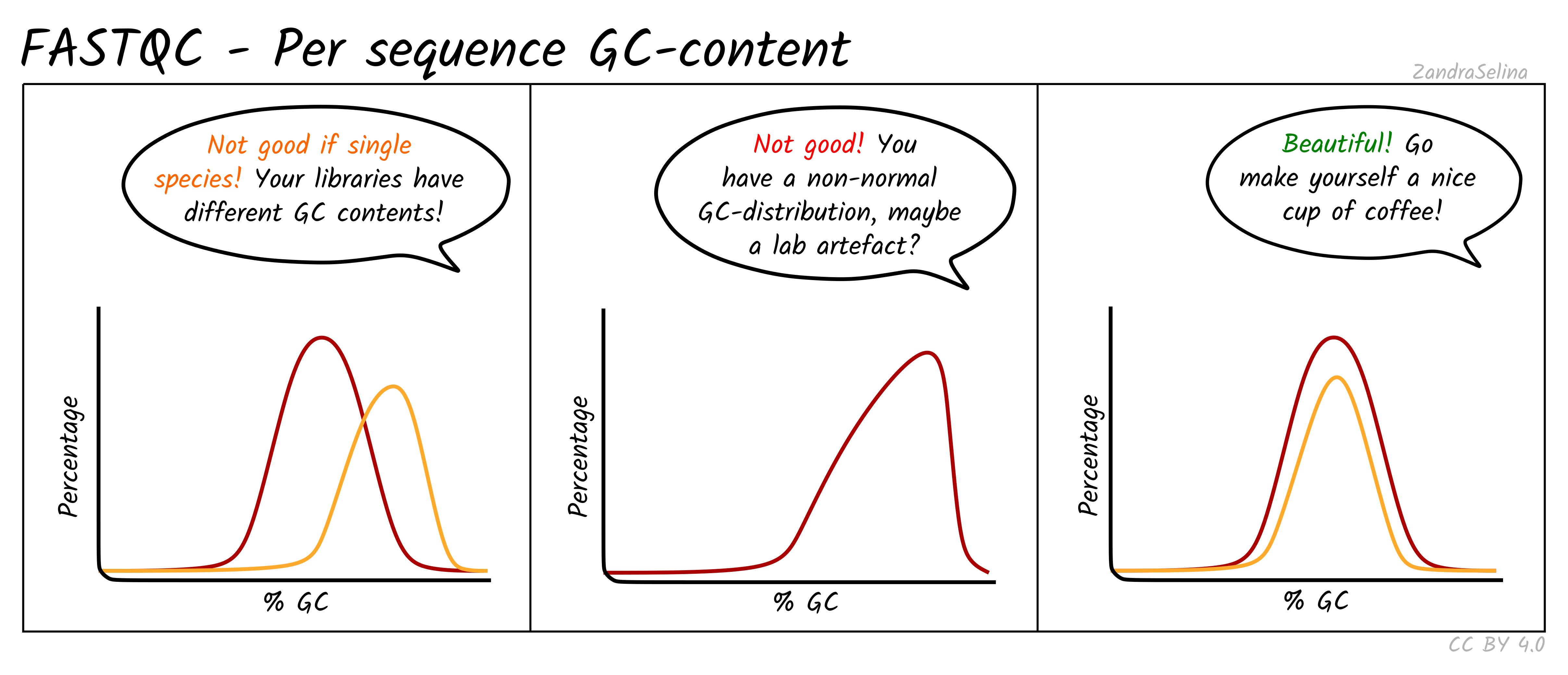
For RNA-seq, mild deviations from a bell curve are normal because expressed transcripts are not GC-neutral. A clearly bimodal curve, however, suggests cross-species contamination.

Adapter Content

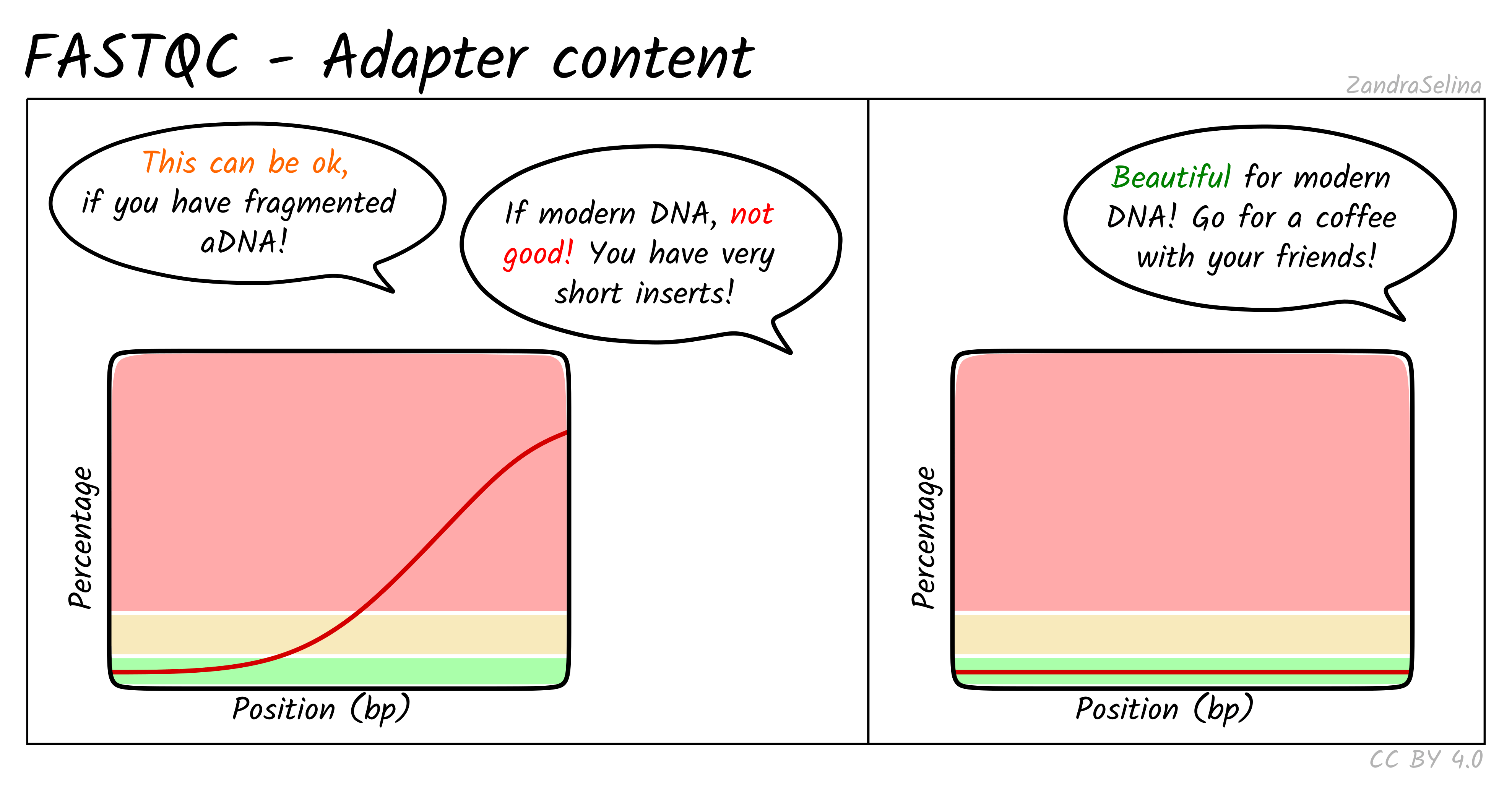
A rising curve at read ends means inserts are shorter than the read length. This is expected for ancient or degraded DNA, but for modern libraries it indicates short fragments that may benefit from trimming.

Sequence Duplication Levels

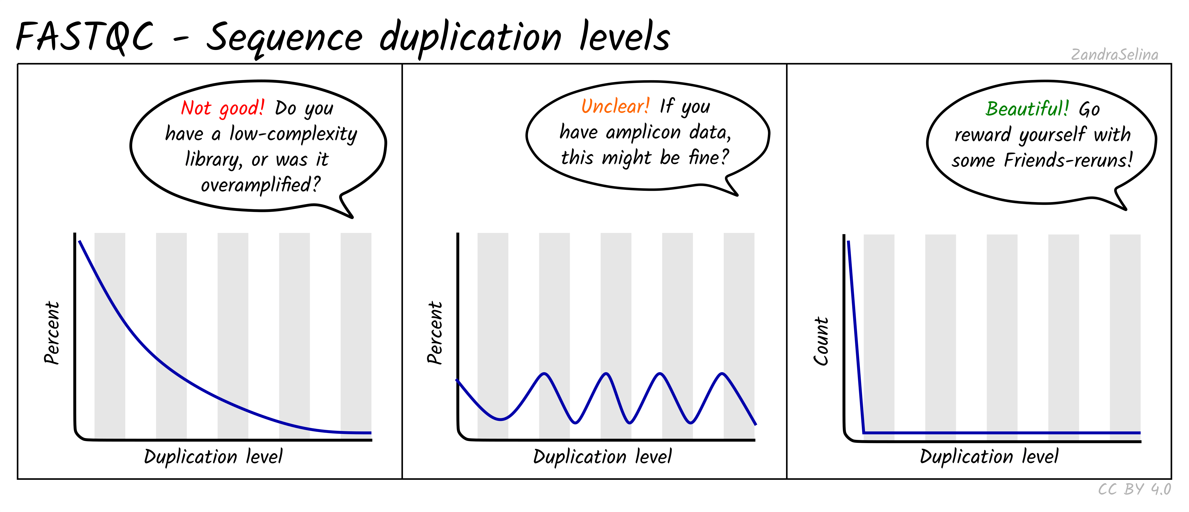
High duplication is expected for RNA-seq (highly expressed genes) and amplicon data, but a heavy tail in WGS points to overamplification or low input material.

Note

For a textual summary of what a problematic sample looks like end-to-end: Q-scores drop below Q20 by position 80-100, adapter content rises to ~25% at the read tail, the Illumina Universal Adapter shows up in overrepresented sequences, the duplication tail is heavy (>30%), and the GC curve has a side shoulder. Any one of these on its own is investigatable; two or more together usually means the sample needs trimming or exclusion.

MultiQC: Aggregating Across Samples

When you have many samples, opening individual FastQC reports one by one is tedious. MultiQC aggregates results from FastQC (and many other tools) into a single interactive HTML report.

1. Load MultiQC:

   module load biocontainers multiqc/1.25.1
   

2. Run MultiQC on all FastQC results:

   mkdir -p multiqc_raw
   multiqc fastqc_raw/ -o multiqc_raw/
   

3. Open multiqc_raw/multiqc_report.html in your browser.

What to Look For in MultiQC

The power of MultiQC is in spotting outliers. When all samples are plotted together:

• General Statistics table: One row per sample showing total reads, %GC, average quality, and % duplicates. Outlier samples stand out immediately.
• Per Base Quality plot: All samples overlaid. Five samples might cluster together with good quality while one sample drops early. That is your problem sample.
• Adapter Content plot: Quickly see which samples have adapter contamination and how severe it is.

The MultiQC status check heatmap gives you a one-glance view of which modules pass, warn, or fail across all samples:

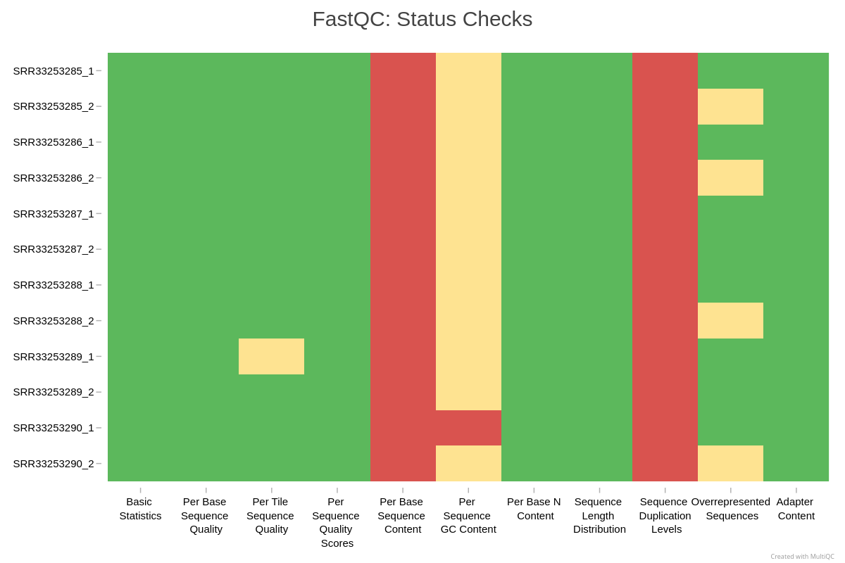
In this example, every sample fails Per Base Sequence Content and Sequence Duplication Levels. For RNA-seq this is expected: random hexamer priming biases the first ~12 bases, and highly expressed transcripts inflate duplication. The Per Sequence GC Content warnings reflect transcriptome composition rather than a library defect. None of these are reasons to discard data.

Tip

MultiQC can aggregate results from dozens of tools, not just FastQC. In later sessions, you can feed it output from fastp, samtools, Picard, STAR, and more to get a comprehensive view of your entire pipeline.

fastp: Trimming and Filtering

fastp is an all-in-one tool for quality filtering, adapter trimming, and read preprocessing. It is fast, handles paired-end data well, and produces its own HTML report.

What Are Adapters?

Adapters are short synthetic DNA sequences added during library preparation. They allow the DNA fragments to attach to the sequencer's flow cell. Adapters are not part of your organism's genome. If a DNA fragment is shorter than the read length, the sequencer reads past the insert and into the adapter on the other side. These adapter sequences need to be removed before analysis.

Running fastp

1. Load fastp:

   module load biocontainers fastp/0.24.0
   

2. Run fastp on a paired-end sample:

   mkdir -p trimmed fastp_reports
   fastp \
       -i raw_reads/sample1_R1.fastq.gz \
       -I raw_reads/sample1_R2.fastq.gz \
       -o trimmed/sample1_R1.trimmed.fq.gz \
       -O trimmed/sample1_R2.trimmed.fq.gz \
       --qualified_quality_phred 20 \
       --length_required 50 \
       --detect_adapter_for_pe \
       --thread 4 \
       --html fastp_reports/sample1.html \
       --json fastp_reports/sample1.json
   

3. Open fastp_reports/sample1.html in your browser to view the before/after quality report.

fastp Parameter Reference

Parameter	Default	Description	When to Change
--qualified_quality_phred	15	Bases below this quality are "unqualified"	Use 20 for standard analysis; 30 for variant calling where accuracy is critical
--unqualified_percent_limit	40	Drop read if this % of bases are unqualified	Lower for stricter filtering
--length_required	15	Discard reads shorter than this after trimming	Use 50 for most Illumina data; adjust based on your aligner's minimum
--detect_adapter_for_pe	off	Auto-detect adapters via paired-end overlap	Always enable for paired-end data
--adapter_sequence	auto	Specify adapter sequence manually	Only if auto-detection fails
--cut_front	off	Sliding window trimming from 5' end	Enable for data with 5' quality issues
--cut_tail	off	Sliding window trimming from 3' end	Enable for data with 3' quality dropoff
--cut_window_size	4	Window size for sliding window trimming	Larger window = more aggressive trimming
--cut_mean_quality	20	Quality threshold for sliding window	Match to your --qualified_quality_phred
--trim_poly_g	auto	Trim poly-G tails	Important for NovaSeq/NextSeq (two-color chemistry artifacts)
--correction	off	Overlap-based error correction for PE reads	Enable for variant calling workflows
--thread	1	Number of processing threads	Use 4 for good performance; fastp is fast even single-threaded

The fastp HTML Report

The fastp report shows:

1. Summary: Total reads before and after filtering, bases before and after, read lengths
2. Quality profiles: Side-by-side before/after quality distribution plots
3. Filtering result: How many reads were removed and why (low quality, too short, too many Ns, adapter contamination)
4. Adapter detection: Which adapter sequences were found and their contamination rate

Note

When NOT to trim aggressively: Modern aligners like BWA-MEM2 and STAR can "soft-clip" low-quality bases at read ends, meaning the aligner ignores bad bases without you removing them. Over-trimming loses data and can introduce biases. For most RNA-seq and WGS workflows, light trimming with fastp defaults is sufficient. Trim adapters (always), apply moderate quality filtering (Q20), and let the aligner handle the rest.

Before/After Comparison

After trimming, run FastQC again on the trimmed reads and use MultiQC to compare raw vs. trimmed results side by side.

1. Run FastQC on trimmed reads:

   mkdir -p fastqc_trimmed
   for fq in trimmed/*.trimmed.fq.gz; do
       fastqc -t 4 -o fastqc_trimmed/ "$fq"
   done
   

2. Run MultiQC on everything (raw FastQC + trimmed FastQC + fastp reports):

   mkdir -p multiqc_combined
   multiqc fastqc_raw/ fastqc_trimmed/ fastp_reports/ -o multiqc_combined/
   

3. Open multiqc_combined/multiqc_report.html and compare:

   • Adapter content: should be gone in trimmed reads
   • Per base quality: 3' end quality should improve (low-quality tails removed)
   • Read counts: some reads were lost during filtering (check fastp statistics)

Is My Data Good Enough?

There is no single universal threshold. What "good enough" means depends on your downstream analysis, your organism, and your experimental design. Here are general guidelines:

Metric	Good	Acceptable	Investigate
% bases Q30+ (after trim)	> 90%	80-90%	< 80%
% adapter content (after trim)	< 1%	1-5%	> 5%
% reads retained after trimming	> 95%	85-95%	< 85%
Duplication rate (WGS)	< 15%	15-30%	> 30%
GC content distribution	Unimodal, matches organism	Slight shoulder	Bimodal

QC Decision Guide

Use this table to decide what action to take based on your QC results:

Scenario	Action
Adapter content > 5%	Trim with fastp (--detect_adapter_for_pe). Re-run FastQC to confirm removal.
Mean quality < Q25	Trim with fastp quality filtering. If still poor, consider re-sequencing.
Quality drops sharply at 3' end	Normal for Illumina. Light trimming with fastp is sufficient.
GC content bimodal	Investigate contamination. Check for mixed species. Consider decontamination tools (e.g., Kraken2).
High duplication in WGS	Low library complexity. May need re-sequencing with more input DNA.
High duplication in RNA-seq	Normal: highly expressed genes produce duplicate reads. Not a QC failure.
Overrepresented adapter sequences	Trim with fastp. Confirm removal with FastQC.
Overrepresented biological sequences	Check what the sequence is (BLAST it). May be rRNA contamination in RNA-seq.
Per base sequence content wobbles at 5' end	Normal: random hexamer priming bias. No action needed.
Very low read count for one sample	Check library prep. May need re-sequencing. Exclude from analysis if insufficient depth.

QC Beyond Raw Reads

Quality control does not end with read trimming. Each stage of your analysis has its own QC metrics.

Alignment QC

After aligning reads to a reference genome (with BWA-MEM2, STAR, HISAT2, etc.), check:

module load biocontainers samtools/1.21

Tool / Command	What It Shows
samtools flagstat sample.bam	Total reads, mapped reads, properly paired reads, duplicates
samtools stats sample.bam	Comprehensive alignment statistics including insert size, error rates
picard CollectAlignmentSummaryMetrics	Mapping rate, mismatch rate, by read group
picard CollectInsertSizeMetrics	Insert size distribution (should match library prep)

Key metrics:

• Mapping rate: > 90% for WGS with good reference; > 70% for RNA-seq
• Duplicate rate: < 30% typical for WGS; higher for low-input libraries
• Insert size: should match your library prep target (e.g., 300-500 bp). Bimodal = problem.
• Properly paired: > 90% expected

Warning

What happens when you skip QC on raw reads? The bad sample (sample6) in our mock data had 68% Q30 bases and 25% adapter content. After trimming, it lost 28% of its reads. After alignment, only 75% of reads mapped (vs. 97% for good samples), and the duplicate rate was 29%. Poor raw data quality cascades through every step.

Variant Calling QC

Metric	Expected Value	What It Means
Ti/Tv ratio (WGS, human)	2.0-2.1	Lower values suggest false positive SNP calls
Ti/Tv ratio (exome, human)	2.8-3.0	Exonic regions have higher Ti/Tv
Het/Hom ratio (human)	1.5-2.0	Very high = contamination; very low = inbreeding or sample issue

RNA-seq Specific QC

After alignment with STAR or HISAT2:

• Read distribution: What fraction maps to exons vs. introns vs. intergenic regions? mRNA-seq should be mostly exonic.
• Gene body coverage: Plot signal from 5' to 3' end of genes. Strong 3' bias = RNA degradation. Strong 5' bias = incomplete reverse transcription.
• Tools: RSeQC, Qualimap, Picard CollectRnaSeqMetrics

Assembly QC

• BUSCO: Checks for expected single-copy orthologs (covered in our HiFi assembly tutorial)
• QUAST: Basic assembly statistics (N50, total length, number of contigs)

Command Cheat Sheet

All commands used in this session in one place:

# --- Setup ---
module --force purge
cd $RCAC_SCRATCH
mkdir -p genomics_exchange/session6
cd genomics_exchange/session6

# --- FastQC on raw reads ---
module load biocontainers fastqc/0.12.1
mkdir -p fastqc_raw
fastqc -t 4 -o fastqc_raw/ raw_reads/*.fastq.gz

# --- MultiQC on raw FastQC results ---
module load biocontainers multiqc/1.25.1
mkdir -p multiqc_raw
multiqc fastqc_raw/ -o multiqc_raw/

# --- Trim with fastp ---
module load biocontainers fastp/0.24.0
mkdir -p trimmed fastp_reports
fastp \
    -i raw_reads/sample1_R1.fastq.gz \
    -I raw_reads/sample1_R2.fastq.gz \
    -o trimmed/sample1_R1.trimmed.fq.gz \
    -O trimmed/sample1_R2.trimmed.fq.gz \
    --qualified_quality_phred 20 \
    --length_required 50 \
    --detect_adapter_for_pe \
    --thread 4 \
    --html fastp_reports/sample1.html \
    --json fastp_reports/sample1.json

# --- FastQC on trimmed reads ---
mkdir -p fastqc_trimmed
fastqc -t 4 -o fastqc_trimmed/ trimmed/*.trimmed.fq.gz

# --- Combined MultiQC report ---
mkdir -p multiqc_combined
multiqc fastqc_raw/ fastqc_trimmed/ fastp_reports/ -o multiqc_combined/

# --- Alignment QC (after aligning with BWA-MEM2 or STAR) ---
module load biocontainers samtools/1.21
samtools flagstat aligned/sample1.sorted.bam
samtools stats aligned/sample1.sorted.bam > sample1.stats.txt

Resources

• FastQC documentation: bioinformatics.babraham.ac.uk/projects/fastqc
• MultiQC documentation: multiqc.info
• fastp paper: Chen et al. (2018). fastp: an ultra-fast all-in-one FASTQ preprocessor. Bioinformatics, 34(17), i884-i890. DOI: 10.1093/bioinformatics/bty560
• RCAC Bioinformatics tutorials: rcac-bioinformatics.github.io
• Genomics Exchange Discord: discord.gg/zEF2nzhXdC
• Questions? Email arun@purdue.edu or rcac-help@purdue.edu

---

Up next: Session 7 (April 21, 2026): Reproducible bioinformatics using Nextflow. We will learn how to wrap QC, alignment, and analysis into reproducible pipelines using Nextflow and nf-core.