Gene prediction using Helixer

Helixer is a deep learning-based gene prediction tool that uses a convolutional neural network (CNN) to predict genes in eukaryotic genomes. Helixer is trained on a wide range of eukaryotic genomes and can predict genes in both plant and animal genomes. Helixer can predict genes without any extrinsic information such as RNA-seq data or homology information, purely based on the sequence of the genome.

1. Installation

Helixer is available as a Singularity container. You can pull the container using the following command:

singularity pull docker://gglyptodon/helixer-docker:helixer_v0.3.3_cuda_11.8.0-cudnn8

This will create helixer_v0.3.3_cuda_11.8.0-cudnn8.sif file in the current directory. We will rename this file to helixer.sif for simplicity.

2. Downloading trained models

Helixer requires a trained model to predict genes. With the included script fetch_helixer_models.py you can download models for specific lineages. Currently, models are available for the following lineages:

• land_plant
• vertebrate
• invertibrate
• fungi

There are instructions to train your own models as well as fine tune the existing models using the RNAseq data for the species of interest. But for this tutorial, we will just use the pre-trained models.

singularity exec helixer.sif fetch_helixer_models.py --all

This will download all lineage models in the models directory. You can also download models for specific lineages using the --lineage option.

The files downloaded will be in the following structure:

models
├── fungi
│   └── fungi_v0.3_a_0100.h5
├── invertebrate
│   └── invertebrate_v0.3_m_0100.h5
├── land_plant
│   └── land_plant_v0.3_a_0080.h5
├── model_list.csv
└── vertebrate
    └── vertebrate_v0.3_m_0080.h5

3. Running Helixer

Helixer requires GPU for prediction. For running Helixer, you need to request a GPU node. You will also need the genome sequence in fasta format. For this tutorial, we will use Maize genome (Zea mays subsp. mays), and use the land_plant model to predict genes.

Download the genome sequence:

wget https://download.maizegdb.org/Zm-B73-REFERENCE-NAM-5.0/Zm-B73-REFERENCE-NAM-5.0.fa.gz
gunzip Zm-B73-REFERENCE-NAM-5.0.fa.gz

Run Helixer:

genome=Zm-B73-REFERENCE-NAM-5.0.fa
species="Zea mays subsp. mays"
output=B73-helixer.gff
singularity exec \
    --bind ${RCAC_SCRATCH} \
    --nv helixer.sif Helixer.py \
    --lineage land_plant \
    --fasta-path ${genome} \
    --species ${species} \
    --gff-output-path ${output}

Note

In A100 GPU nodes, the run time for predicting genes in Maize genome takes around 3.5 hours (03:36:23), with 6 CPUs --ntasks-per-node=6. The memory usage was 7.98 GB.

The GFF format output had 41,923 genes predicted using Helixer. You can view the various features in the gff file using the following command:

grep -v "^#" B73-helixer.gff | cut -f 3 | sort | uniq -c

outputs:

2,19,488  CDS
2,41,560  exon
  52,607  five_prime_UTR
  41,923  gene
  41,923  mRNA
  52,298  three_prime_UTR

Warning

As you may have noticed, the number of mRNA and gene features are the same. This is because isoforms aren't predicted by Helixer and you only have one transcript per gene. Exons are identified with high confidence and alternative isoforms are usually collapsed into a single gene model.

4. Comparing and benchmarking

We will download the reference annotations for Maize genome from MaizeGDB and compare the predicted genes with the reference annotations.

wget https://download.maizegdb.org/Zm-B73-REFERENCE-NAM-5.0/Zm-B73-REFERENCE-NAM-5.0.gff3.gz
gunzip Zm-B73-REFERENCE-NAM-5.0.gff3.gz

Processing GFF output

The output generated by Helixer is in GFF format. However we might have to format it further to make it compatible with our processing workflow. Here are the steps to process the GFF output:

# sanitize the gff3 file
ml purge
ml biocontainers
ml genometools
gff3_file=B73-helixer.gff
gt gff3 \
    -sort \
    -tidy \
    -setsource "helixer" \
    -force -o B73-helixer_gt.gff3 \
    ${gff3_file}

# standardize
ml purge
ml biocontainers
ml agat
agat_convert_sp_gxf2gxf.pl \
    -g B73-helixer_gt.gff3 \
    -o B73-helixer_v1.0.gff3

# extract CDS and PEP sequences
ml purge
ml biocontainers
ml cufflinks
gffread B73-helixer_v1.0.gff3 \
    -g Zm-B73-REFERENCE-NAM-5.0.fa \
    -x B73-helixer_v1.0.cds.fasta \
    -y B73-helixer_v1.0.pep.fasta

A. BUSCO profiling

We will use BUSCO to profile the predicted genes and reference annotations.

ml biocontainers
ml busco
busco \
    -i B73-helixer_v1.0.pep.fasta \
    -c ${SLURM_CPUS_ON_NODE} \
    -o B73-helixer_v1.0_busco \
    -m prot \
    -l poales_odb10 \
    -f

We will also do this on the original reference annotations as well as the genome sequence.

Reference genome:

# reference genome
busco \
    -i Zm-B73-REFERENCE-NAM-5.0.fa \
    -c ${SLURM_CPUS_ON_NODE} \
    -o Zm-B73-REFERENCE-NAM-5.0_busco \
    -m genome \
    -l poales_odb10 \
    -f

Reference annotations:

# reference annotations
wget https://download.maizegdb.org/Zm-B73-REFERENCE-NAM-5.0/Zm-B73-REFERENCE-NAM-5.0_Zm00001eb.1.protein.fa.gz
gunzip Zm-B73-REFERENCE-NAM-5.0_Zm00001eb.1.protein.fa.gz
busco \
    -i Zm-B73-REFERENCE-NAM-5.0_Zm00001eb.1.protein.fa \
    -c ${SLURM_CPUS_ON_NODE} \
    -o Zm-B73-REFERENCE-NAM-5.0_protein_busco \
    -m prot \
    -l poales_odb10 \
    -f

Once the BUSCO profiling is done, the results can be compared.

Table 1: BUSCO results

Category	Helixer	B73.v5 (MaizeGDB)	B73.v5 (Reference)
Complete BUSCOs	4,808 (98.2%)	4,729 (96.6%)	4,807 (98.2%)
Single-Copy BUSCOs	4,053 (82.8%)	2,123 (43.4%)	4,053 (82.8%)
Duplicated BUSCOs	755 (15.4%)	2606 (53.2%)	754 (15.4%)
Fragmented BUSCOs	34 (0.7%)	39 (0.8%)	10 (0.2%)
Missing BUSCOs	54 (1.1%)	128 (2.6%)	79 (1.6%)
Total BUSCOs	4,896	4,896	4,896

or visualized as a stacked bar plot:

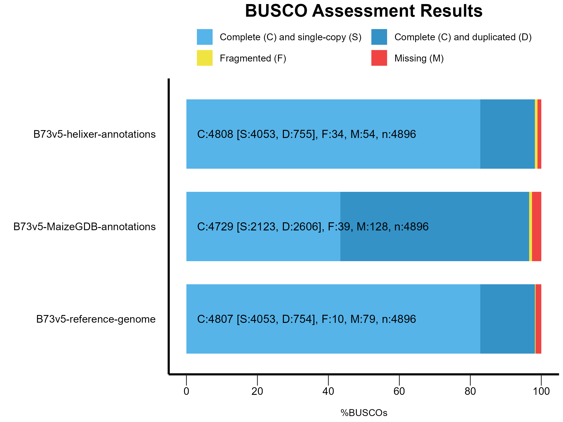
Figure 1: BUSCO results for Helixer, B73.v5 (MaizeGDB) and B73.v5 (Reference) annotations.

Note

The Helixer predictions shows higher number of complete BUSCOs (single-copy + duplicated) than current B73.v5 annotations available at MaizeGDB. It also reports only 54 missing BUSCOs, lowest among all 3 BUSCO results meaning it was able to recover more BUSCO genes than what BUSCO software could predict/recover using AUGUSTUS/tblastn search!

Warning

The duplicated genes in B73.v5 (MaizeGDB) should not be interpreted as paralogs. Since we did not use just primary transcripts for running BUSCO, the alternative isoforms of the same gene are reported as "duplicated".

B. Comparing annotations

We will use mikado to compare the annotations. Mikado is a tool to compare and merge gene annotations. We will use the mikado compare command to compare the annotations. We will filter V5 annotations to only include primary transcripts and only compare protein coding genes.

conda activate mikado
mikado compare \
    --protein-coding \
    -r B73.v5_primary-only.gff3 \
    -p B73-helixer_v1.0.gff3 \
    -o ref_NAM.B73v5-vs-prediction_HELIXERv1_compared \
    --log compare.log

The output will be in the ref_NAM.B73v5-vs-prediction_HELIXERv1_compared directory. The summary.tsv file will have the comparison results.

Table 2: Mikado comparison results

Comparison Level	Sensitivity (Sn)	Precision (Pr)	F1 Score
Base level	81.90%	75.29%	78.46%
Exon level (stringent)	53.21%	42.82%	47.46%
Exon level (lenient)	75.93%	61.02%	67.66%
Splice site level	85.06%	65.89%	74.26%
Intron level	78.45%	60.77%	68.49%
Intron chain level (stringent)	38.10%	32.85%	35.28%
Transcript level (>=80% base F1)	36.89%	34.98%	35.91%
Gene level (>=80% base F1)	36.89%	34.98%	35.91%

Note

When compared against each other, the Helixer predictions, at base level, matches the B73.v5 (maizeGDB annotations) really well. However, the precision is lower for Helixer predictions, likely because there are higher number of novel genes predicted in Helixer that are non existant in B73.v5 annotations.

Table 3: Summary of comparison

Feature	Total Count	Missed Count (%)	Novel Count (%)
Transcripts	39,756	7,539 (18.96%)	8,306 (19.81%)
Genes	39,756	7,539 (18.96%)	8,306 (19.81%)

Note

The Helixer predictions missed 7,359 predictions (out of 39,756) that were in B73.v5, but also predicted 8,306 novel transcripts. Since Helixer does not predict isoforms, the number of genes and transcripts are the same.

C. Feature assignment

B73 has extensive expression data and this can be used to evaluate the gene predictions. If the annotations are accurate, more RNA-seq reads will align within the predicted features, making a higher proportion of assigned reads an indicator of annotation accuracy. Similarly, higher proportions of unassigned reads indicate potential inaccuracies in the annotations, suggesting that important features may be missing or incorrectly predicted.

Expression data for B73 was downloaded from MaizeGDB (as BAM files) and feature assignment was done using featureCounts from the subread package (both NAM.v5 and Helixer predictions).

ml biocontainers
ml subread
featureCounts \
    -T 8 \
    -a Zm-B73-REFERENCE-NAM-5.0_Zm00001eb.1.gff3 \
    -o v5.str2 \
    -s 2 \
    -p --countReadPairs \
    -t gene -g ID \
    --tmpDir /dev/shm \
    *.bam &> v5_gene-str2_PE.stdout

featureCounts \
    -T 8 \
    -a B73-helixer_v1.0.gff3 \
    -o helixer.str2 \
    -s 2 \
    -p --countReadPairs \
    -t gene -g ID \
    --tmpDir /dev/shm \
    *.bam &> helixer_gene-str2_PE.stdout

Assigned FeaturesUnassigned Features

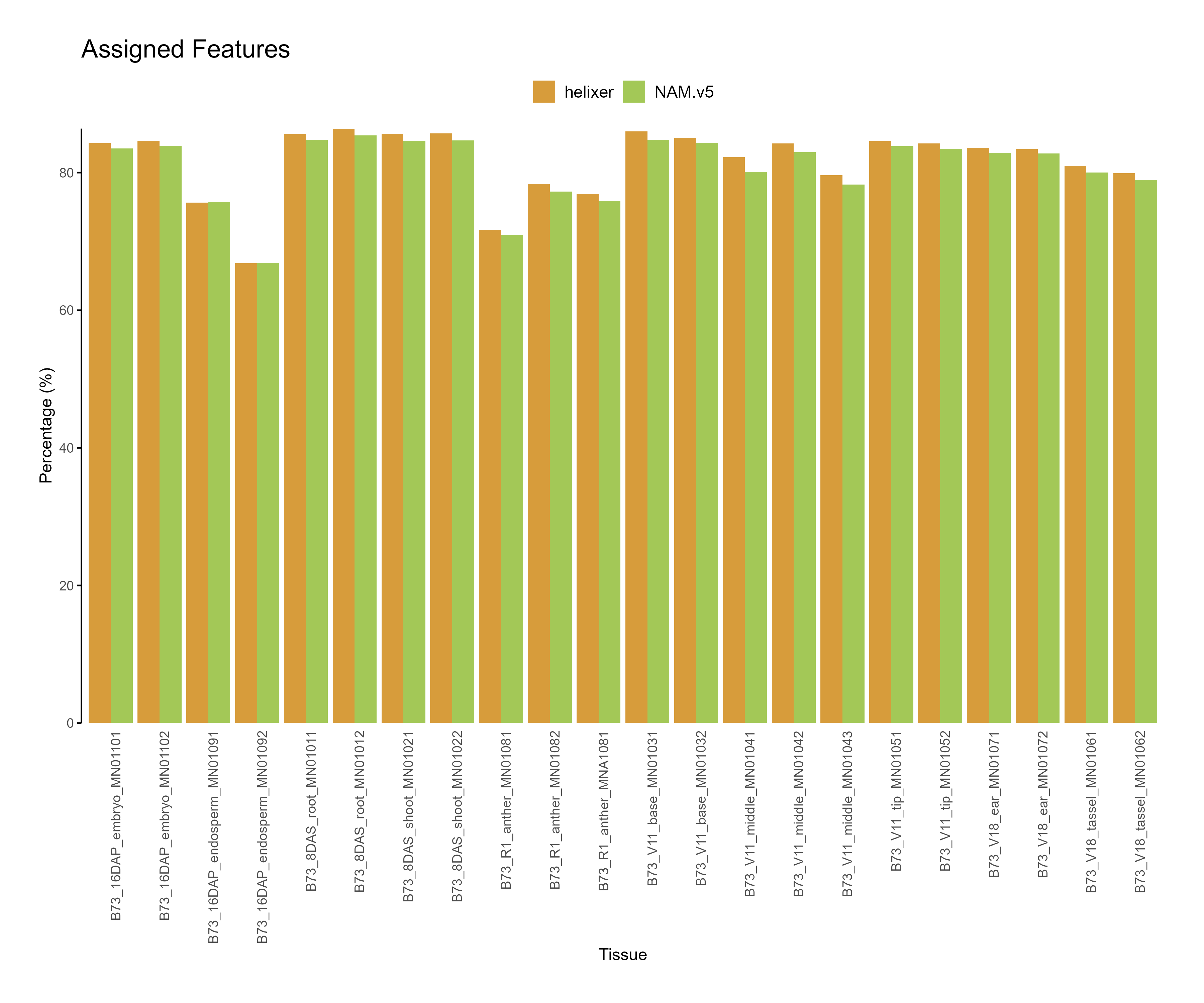
Figure 2: Feature assignment for B73.v5 and Helixer predictions. The reads assigned to helixer features are higher across tissues as compared to NAM.v5 annotations.

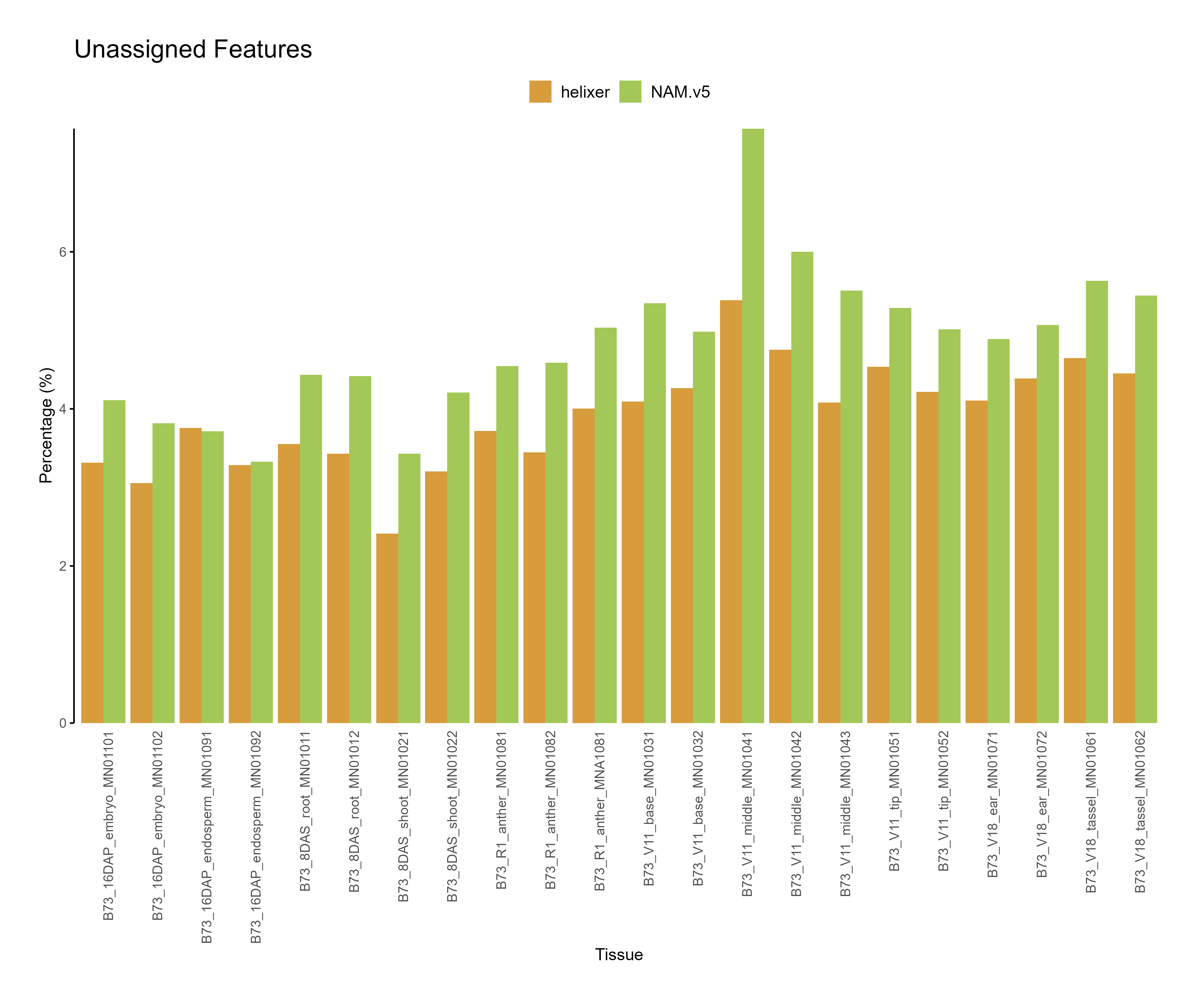
Figure 3: Feature assignment for B73.v5 and Helixer predictions. The unassigned reads are higher for NAM.v5 annotations across tissues.

The code used for parsing featureCounts summary files and generating the plots can be found here: parse_subreads.R

Note

The slightly higher assignment rate for Helixer predictions suggests that the predictions are capturing more coding regions of the genome. Similarly, lower unassigned reads indicate Helixer predictions have better accuracy than current annotations. For differential gene expression studies, higher assignment rates are desirable as they indicate more accurate gene models.

D. Functional annotation

The Eukaryotic Non-Model Transcriptome Annotation Pipeline (EnTAP) can be used for functional annotation of the predicted genes. We will use the entap pipeline determine proportion of genes with functional annotations in each predictions.

ml purge
ml anaconda
conda activate entap
for cds in B73-helixer_v1.0.cds.fasta Zm-B73-REFERENCE-NAM-5.0_Zm00001eb.1.cds.fa; do
EnTAP \
    --runP \
    -i ${cds} \
    -d ${RCAC_SCRATCH}/entap_db/bin/ncbi_refseq_plants.dmnd \
    -d ${RCAC_SCRATCH}/entap_db/bin/uniprot_sprot.dmnd  \
    -t ${SLURM_CPUS_ON_NODE} \
    --ini ${RCAC_SCRATCH}/entap_db/entap_config.ini
done

Percent identityCoding frame with gene functionCoding frame with pfam domain

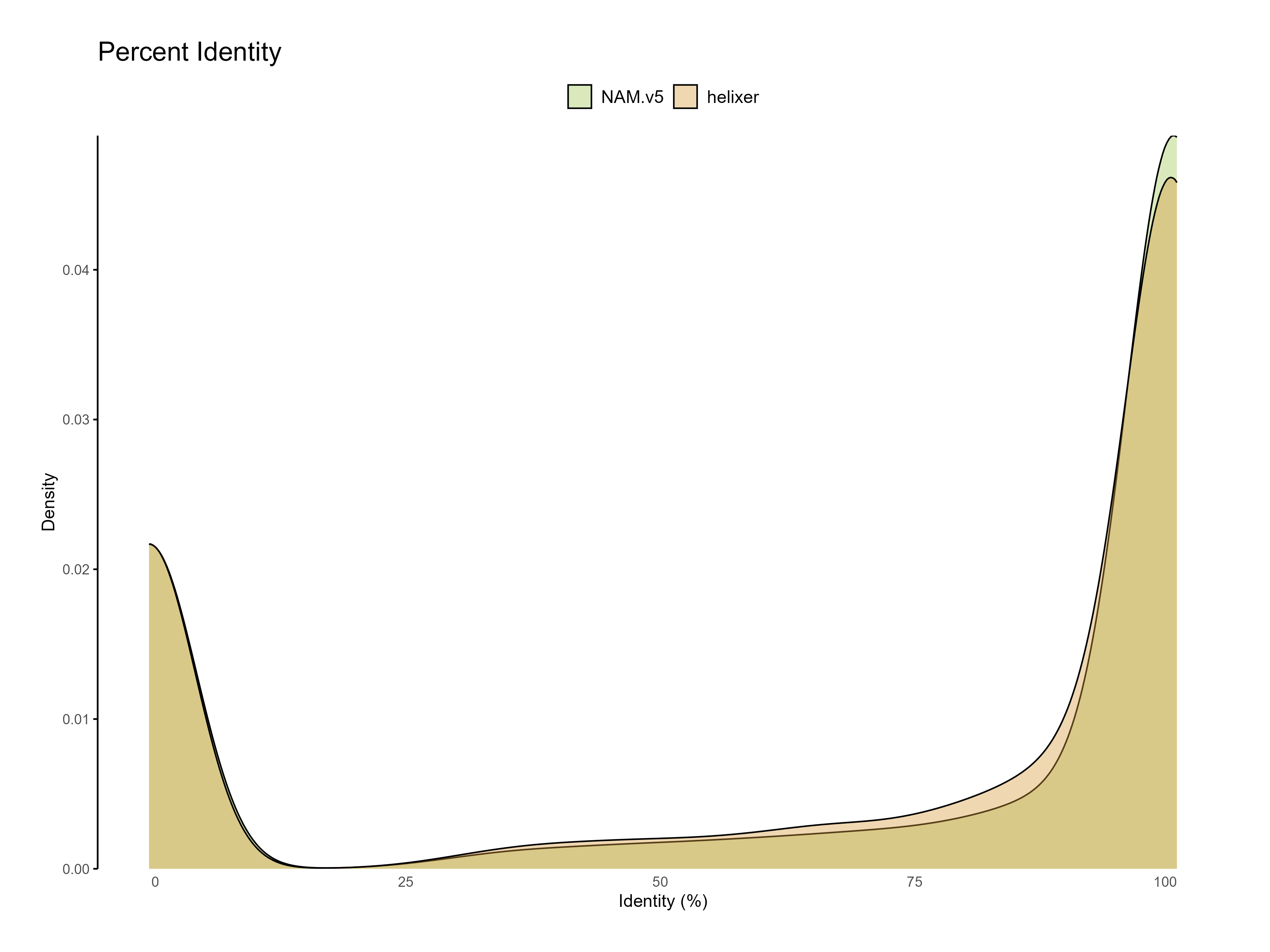
Figure 4: Percent identity of each predicted gene to the reference databases sequences (one hit per query).

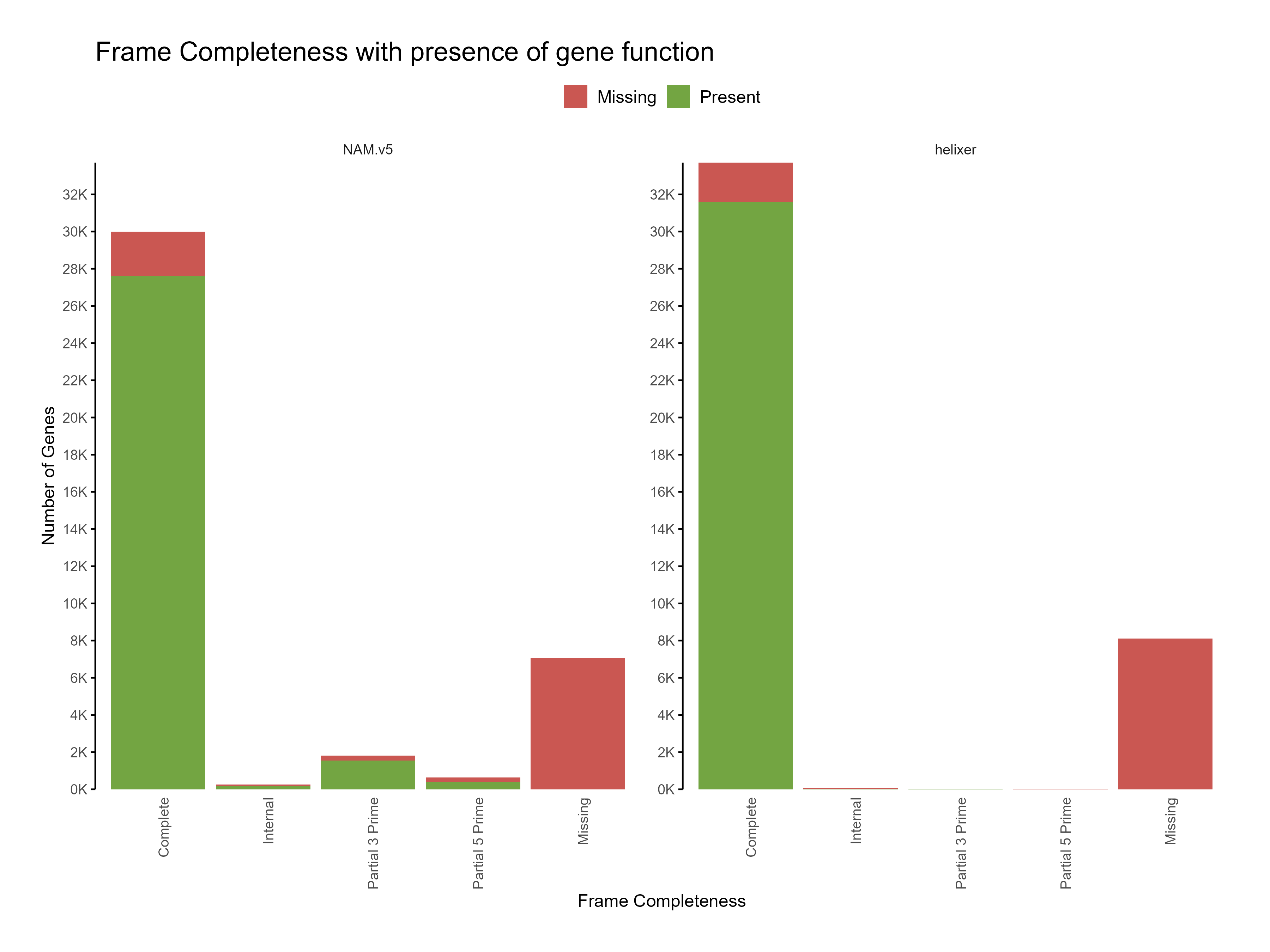
Figure 5: Distribution of frame completeness with presence of gene function across predictions

Figure 5: Distribution of frame completeness with presence of pfam domains across predictions

The code used for parsing EnTAP's entap_results.tsv files and generating the plots can be found here: parse_subreads.R

Note

The functional annotation results show that the Helixer predictions have higher proportion of genes with functional annotations compared to the reference annotations. Predictions with similarity to existing sequences in the databases are likely to be more accurate than those without any similarity.

E. Phylostrata analysis

Phylostrata analysis can be used to determine the evolutionary age of the predicted genes. We will use the phylostrata package to determine the phylostrata of the predicted genes.

countspercent

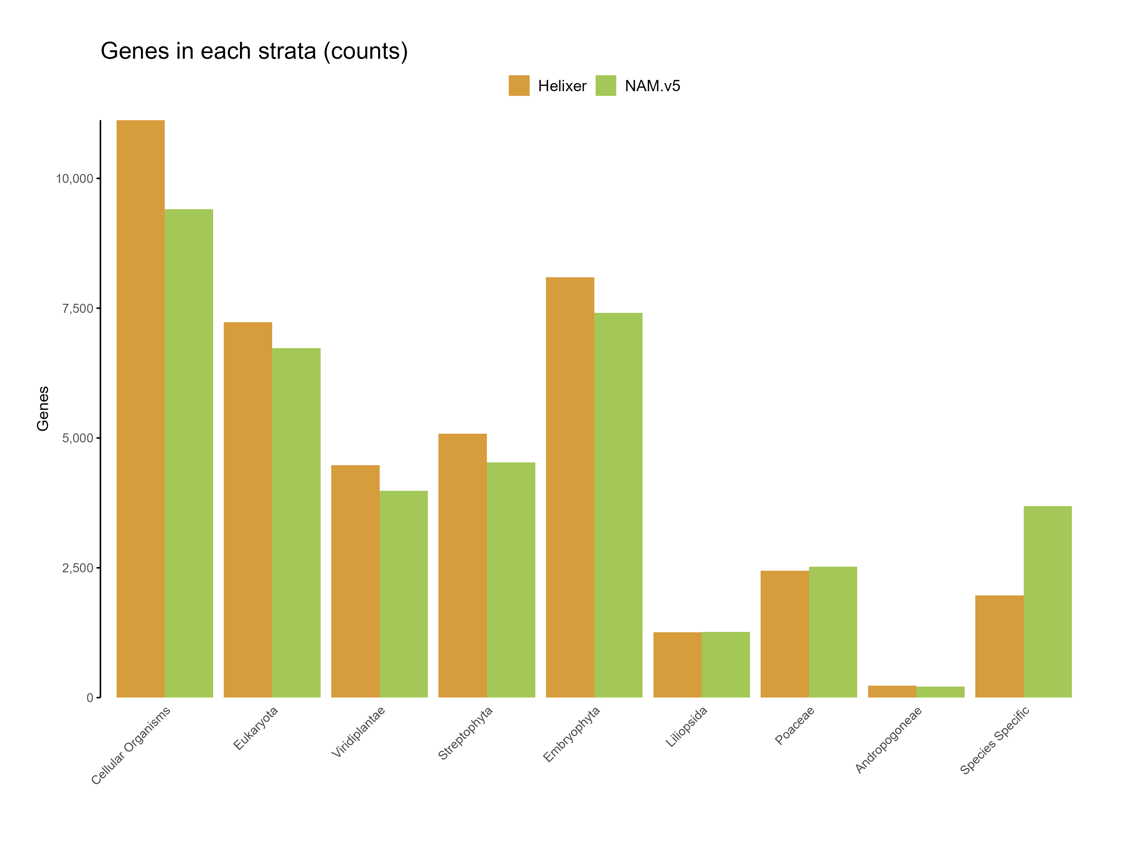
Figure 6: Genes in each strata for the predictions (count)

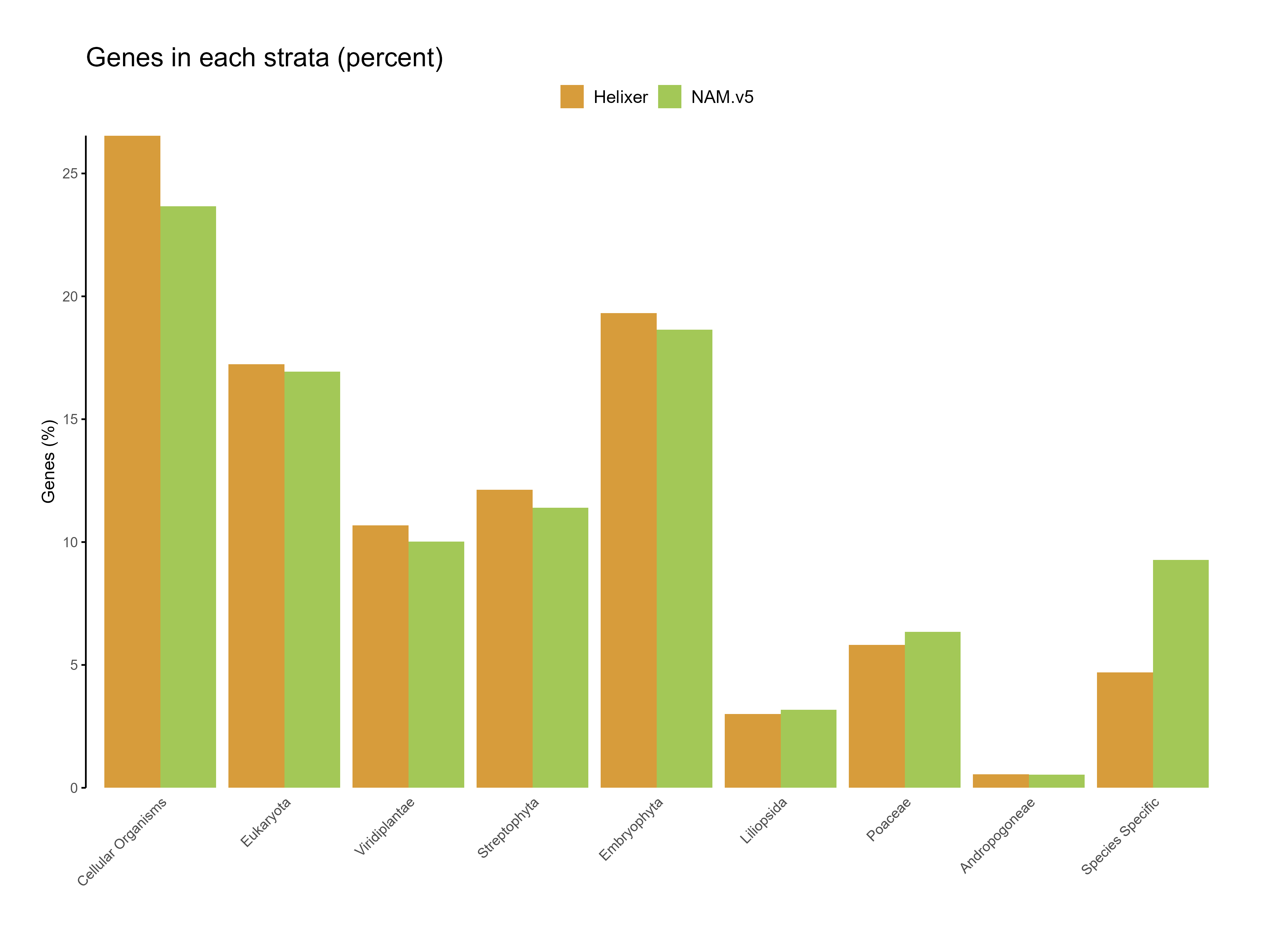
Figure 7: Genes in each strata for the predictions (percent)

The code used for parsing phylostrata analyses (phylostrata_run.R) and for plotting results (phylostrata_plot.R) are provided in the repository.

Note

The higher proportion of genes in deeply conserved phylostrata (e.g., cellular organisms and eukaryota) underscores Helixer's strength in accurately identifying core, evolutionarily conserved genes. This alignment with conserved regions can be interpreted as strong evidence of the model's reliability in identifying well-established gene structures.

Warning

Limitations in Novel Gene Identification: The relatively low representation in species-specific phylostrata suggests that Helixer may struggle with genes that are unique or novel to a particular species. This could be due to the lack of specific training data for these novel genes or the limitations of the model in detecting sequences that deviate from conserved gene structures.

F. GFF3 stats comparison

You can generate comprehensive statistics for the GFF3 files using the agat_sp_statistics.pl script from the agat package.

ml biocontainers
ml agat
agat_sp_statistics.pl \
    -g B73-helixer_v1.0.gff3 \
    -o B73-helixer_v1.0.stats
agat_sp_statistics.pl \
    -g Zm-B73-REFERENCE-NAM-5.0.gff3 \
    -o Zm-B73-REFERENCE-NAM-5.0.stats

The statistics can be compared to identify differences in the gene predictions.

G. OMArk proteome assessment

OMArk provides measures of proteome completeness, characterizes the consistency of all protein coding genes with regard to their homologs, and identifies the presence of contamination from other species

OMArk for NAM.v5OMArk for Helixer

omark_sif="${RCAC_SCRATCH}/omark/omark_0.3.0--pyh7cba7a3_0.sif"
peptide="${RCAC_SCRATCH}/omark/Zm-B73-REFERENCE-NAM-5.0_Zm00001eb.1.protein.fa"
database="${RCAC_SCRATCH}/omark/LUCA.h5"
apptainer exec ${omark_sif} omamer search \
    --db ${database} \
    --query ${peptide} \
    --out ${peptide%.*}.omamer \
    --nthreads ${SLURM_CPUS_ON_NODE}
# only needed for NAM.v5
grep ">" ${peptide} |\
    sed 's/>//g' |\
    awk -F_ '{a[$1] = a[$1] ? a[$1]","$0 : $0} END {for (i in a) print a[i]}' > ${peptide%.*}.splice
apptainer exec ${omark_sif} omark \
    --file ${peptide%.*}.omamer \
    --database ${database} \
    --outputFolder ${peptide%.*} \
    --og_fasta ${peptide} \
    --isoform_file ${peptide%.*}.splice

omark_sif="${RCAC_SCRATCH}/omark/omark_0.3.0--pyh7cba7a3_0.sif"
peptide="${RCAC_SCRATCH}/omark/helixer_pep.fa"
database="${RCAC_SCRATCH}/omark/LUCA.h5"
apptainer exec ${omark_sif} omamer search \
    --db ${database} \
    --query ${peptide} \
    --out ${peptide%.*}.omamer \
    --nthreads ${SLURM_CPUS_ON_NODE}
apptainer exec ${omark_sif} omark \
    --file ${peptide%.*}.omamer \
    --database ${database} \
    --outputFolder ${peptide%.*} \
    --og_fasta ${peptide} \
    --isoform_file ${peptide%.*}.splice

Table 4: Conserved HOGs analysis for completeness assessment of gene sets in Helixer and NAM.v5 This table provides a completeness assessment of the gene sets for both Helixer and NAM.v5 based on conserved Hierarchical Orthologous Groups (HOGs) within the Panicoideae clade. The categories include the number of single-copy genes, duplicated genes, and missing genes, with a distinction between expected and unexpected duplications. The assessment serves as a proxy for evaluating the gene repertoire completeness and duplication events in each dataset.

Category	Helixer Count	Helixer (%)	NAM.v5 Count	NAM.v5 (%)
Single	13,072	63.75%	9,150	44.62%
Duplicated	5,874	28.65%	2,240	10.92%
Duplicated, Unexpected	2,150	10.49%	990	4.83%
Duplicated, Expected	3,724	18.16%	1,250	6.10%
Missing	1,559	7.60%	9,115	44.45%
Total HOGs	20,505	100.00%	20,505	100.00%

Table 5: Consistency assessment of annotated protein-coding genes in Helixer and NAM.v5 proteomes. This table presents the consistency assessment of annotated protein-coding genes within the Helixer and NAM.v5 proteomes. The categories evaluate gene placements as "Consistent" with the ancestral lineage, "Inconsistent" (potential misannotations), "Contaminants" (genes from other lineages), and "Unknown" (unmatched genes). Subcategories include partial hits and fragmented proteins, which may indicate issues with gene models, annotation, or sequence integrity.

Category	Helixer Count	Helixer (%)	NAM.v5 Count	NAM.v5 (%)
Total Proteins	41,923	100.00%	39,756	100.00%
Consistent	38,997	93.02%	20,208	50.83%
Consistent, partial hits	5,412	12.91%	3,541	8.91%
Consistent, fragmented	3,094	7.38%	2,627	6.61%
Inconsistent	757	1.81%	1,910	4.80%
Inconsistent, partial hits	291	0.69%	335	0.84%
Inconsistent, fragmented	279	0.67%	921	2.32%
Contaminants	0	0.00%	0	0.00%
Contaminants, partial hits	0	0.00%	0	0.00%
Contaminants, fragmented	0	0.00%	0	0.00%
Unknown	2,169	5.17%	17,638	44.37%

H. CDS assessments (GC, length, start/stop)

We can use bioawk get relevant stats on the CDS sequences predicted by Helixer and compare them with the reference annotations.

for f in *_cds.fa; do
    bioawk -c fastx 'BEGIN{OFS="\t"}{
    print $name,length($seq),gc($seq),substr($seq,0,3),reverse(substr(reverse($seq),0,3))
    }' $f > ${f%.*}.info;
done

The plots were generated using the following R script: cds_assesment.R

CDS lengthGC contentCodon type

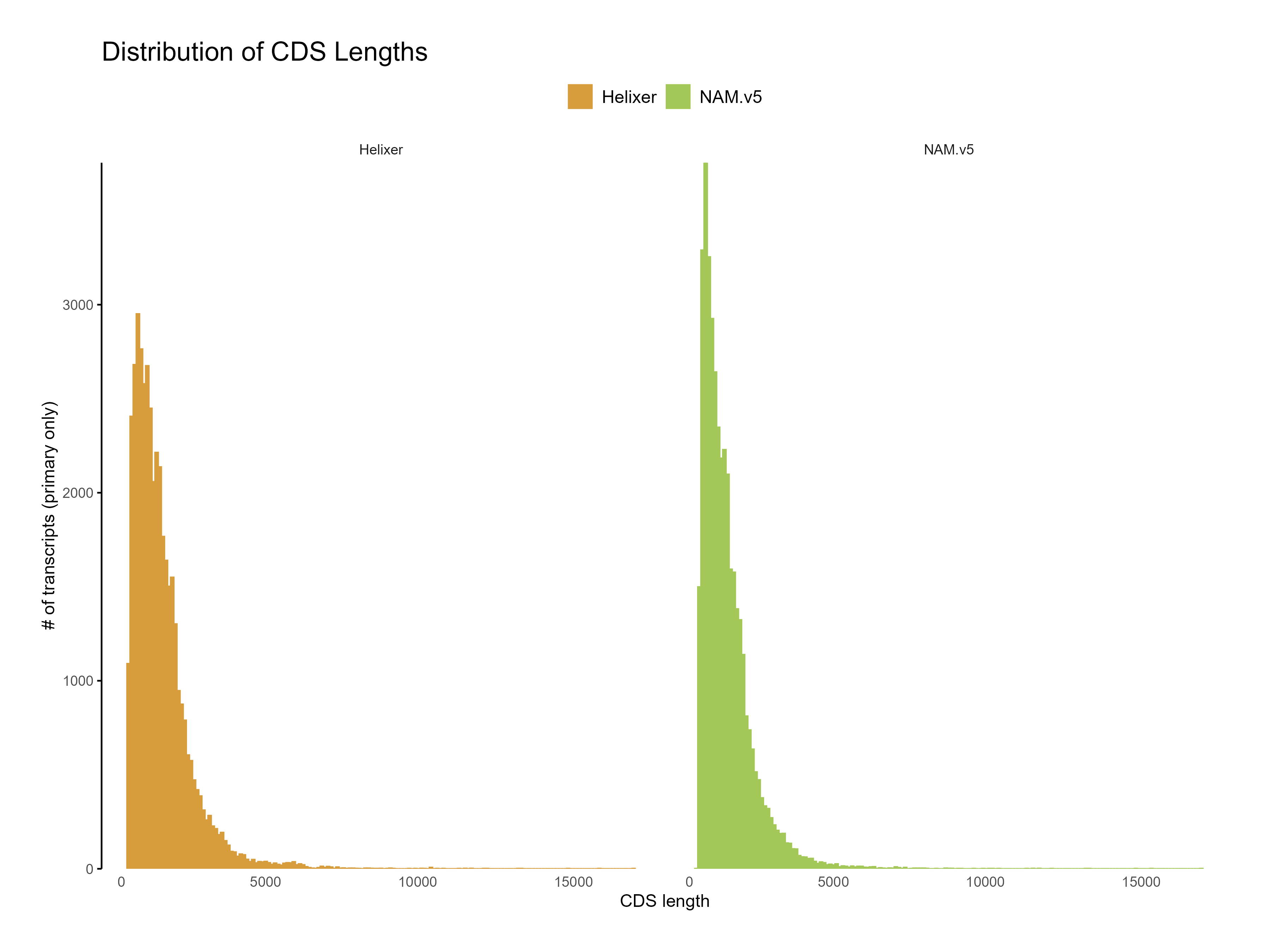
Figure 8: Distribution of CDS length for Helixer and NAM.v5 predictions. The Helixer predictions have a lower proportion of shorter CDS lengths compared to NAM.v5 annotations.

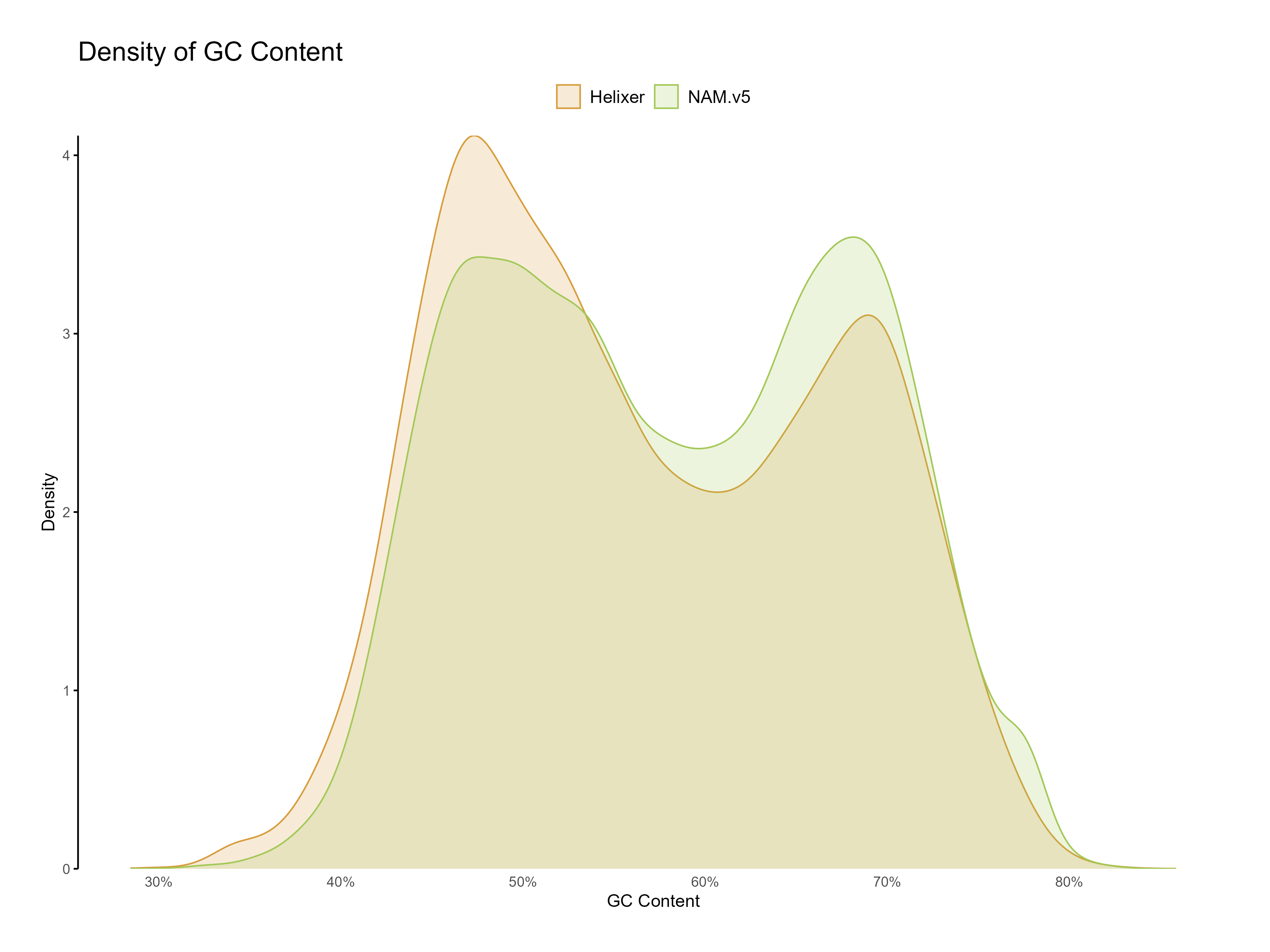
Figure 9: Distribution of GC content for Helixer and NAM.v5 predictions. Both predictions have a classic dual GC peak typical to grasses.

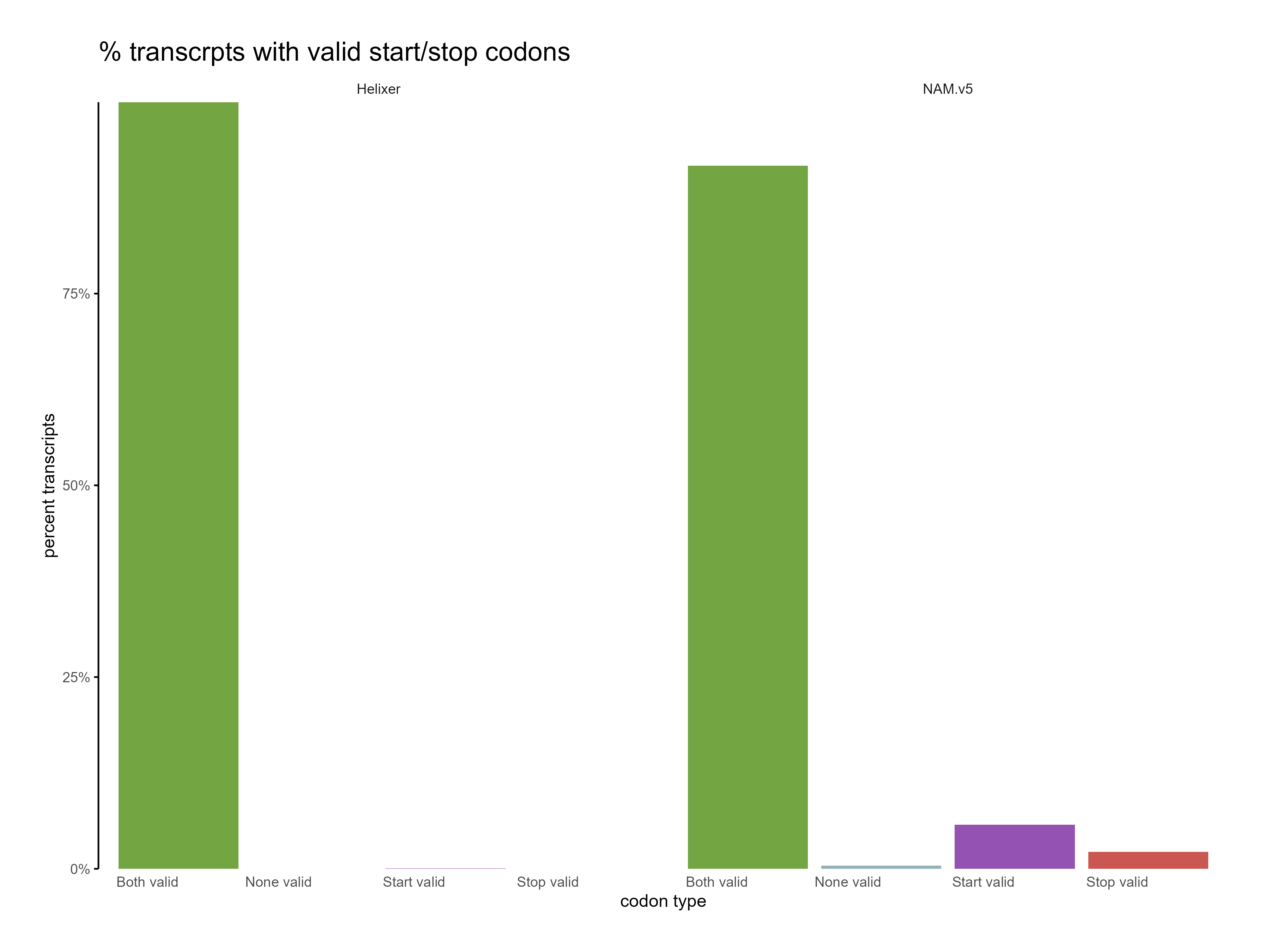
Figure 10: Distribution of start and stop codons for Helixer and NAM.v5 predictions. The Helixer predictions have a higher proportion of valid start and stop codons.

Key Points

1. Helixer's strength in conserved genes: Helixer effectively predicts genes in deeply conserved phylostrata, indicating strong performance in identifying core, evolutionarily stable genes across eukaryotic lineages.

2. Limited novel gene detection: Helixer shows lower accuracy in detecting species-specific genes, suggesting that identifying novel or rapidly evolving genes may not be its primary strength.

3. Pre-trained models for versatile Use: With pre-trained models for various lineages (plants, animals, fungi), Helixer is accessible for multiple research applications without requiring additional RNA-seq or homology data.

4. Simplicity of Gene Prediction: Helixer allows for rapid and straightforward gene prediction with a single command, requiring no external data or repeat masking. It can predict genes in complex, highly repetitive genomes like maize in under four hours. This simplicity, combined with easy installation, has the potential to revolutionize gene prediction workflows.

5. Ideal for Comparative Genomics: Helixer's robust detection of conserved genes makes it a valuable tool for studies focused on comparative genomics and understanding fundamental gene functions.

6. Potential for Improvement: The presence of unassigned reads across samples and limited species-specific gene detection highlight areas for future model refinement, possibly with custom training for novel species.

Warning

Helixer requires GPU for prediction to run efficiently. The prediction time can vary based on the size of the genome and the complexity of the gene structures.

5. References

• Helixer GitHub

• Helixer Webtool

• Holst F, Bolger A, Gunther C, Mass J, Kindel F, Triesch S, Kiel N, Saadat N, Ebenhoh O, Usadel B,Schwacke R, Bolger M, Weber APM, Denton AK Helixer - de novo prediction of primary eukaryotic gene models combining deep learning and a Hidden Markov Model. bioRxiv. 2023 Feb 06: 2023.02.06.527280. Preprint. (not been certified by peer review)

• Stiehler F, Steinborn M, Scholz S, Dey D, Weber APM, Denton AK Helixer: cross-species gene annotation of large eukaryotic genomes using deep learning. Bioinformatics. 2020 Dec, 36(22-23): 5291-5298.