GeMoMa to merge annotations
-
Prerequisites
- Target genome assembly (
fastaformat) - we will use B73.v5 genome - ab initio predictions (
.gff3format) - we will use Helixer output - Homology predictions (
.gff3format) - Sorghum and B97 annotations
- Target genome assembly (
-
Software
- GeMoMa (version >= 1.9 recommended)
- Dependencies:
java >1.8,blastormmseqs
GeMoMa overview
Gene Model Mapper (GeMoMa) is a homology-based gene prediction tool that transfers protein-coding gene models from one or more reference genomes to a target genome. It can incorporate RNA-seq evidence, filter predictions using customizable criteria, and merge multiple annotations--including ab initio and transcriptome-based predictions--into a unified gene set.
Use case: merging annotations
Helixer is a deep learning-based predictor that provides accurate gene predictions from genome sequence alone. However, it does not predict alternative isoforms and tends to collapse all transcript variants into a single flattened gene model, especially in regions with overlapping exons or alternative splicing.
Homology predictions can be used to recover these missing isoforms and provide additional context for gene structure. GeMoMa excels at this task by leveraging evolutionary conservation across related species, allowing it to transfer annotations from well-annotated genomes to the target genome.
By merging Helixer predictions with GeMoMa:
- You retain Helixer's high confidence gene boundaries and structure for primary transcripts.
- You recover missing isoforms and splice variants that Helixer collapses.
- You gain orthology-supported annotation refinement using multiple maize lines and related species like Sorghum bicolor.
- You generate a more complete and biologically realistic gene set, even without long-read or isoform-resolving RNA-seq data.
This hybrid strategy takes advantage of both machine learning accuracy and evolutionary conservation to compensate for the limitations of any single method.
Warning
GeMoMa does not predict UTRs well without evidence. Despite Helixer providing UTR predictions, GeMoMa tries to compute UTRs based on the predicted CDS, which can lead to inaccuracies.
Input preparation
In this example, for the B73.v5 genome, we will merge ab initio predictions obtained from Helixer with the homology predictions of its close relatives (Maize inbred B97 and Sorghum).
- Download target genome - this is the genome we will be annotating with GeMoMa:
- Download Helixer predictions - these are the ab initio predictions we will be merging with GeMoMa:
- Download homology predictions (genome and gff3 files) - these are the annotations from related species that will be used to inform GeMoMa:
- Unzip the downloaded files:
Setup GeMoMa
GeMoMa is executed using a Java-based CLI pipeline. Here we will run GeMoMa with the target genome, Helixer predictions, and homology-based annotations from related species. We will generate a merged annotation file in GFF3 format.
We will install GeMoMa using BioConda:
Run GeMoMa
Save this script as run_gemoma.sh and run it in a terminal with the command:
The options used in the command above are:
| Option | Explanation |
|---|---|
t=$genome |
Target genome (FASTA) to annotate. |
s=own |
Reference species data will be extracted by GeMoMa from annotation + genome. |
i=sb |
Identifier for reference species (Sorghum bicolor). |
a=$sorghumGFF |
GFF3 gene annotation for Sorghum bicolor. |
g=$sorghumFa |
FASTA genome for Sorghum bicolor. |
i=zm |
Identifier for second reference species (e.g., maize B97). |
a=$maize1GFF3 |
GFF3 gene annotation for maize B97. |
g=$maize1 |
FASTA genome for maize B97. |
ID=helixer |
Unique label for Helixer-based annotation source. |
e=$helixer |
External GFF3 annotation to be merged (Helixer output). |
AnnotationFinalizer.u= |
Disable UTR prediction (no RNA evidence available). |
AnnotationFinalizer.r=SIMPLE |
Rename gene/transcript IDs using a simple prefix-based system. |
AnnotationFinalizer.p=$name |
Prefix used in renaming genes and transcripts. |
AnnotationFinalizer.n=true |
Add new names as Name= attributes in GFF3 output. |
sc=false |
Disable synteny check. |
o=false |
Do not write individual predictions per reference species. |
p=true |
Output predicted proteins as FASTA. |
pc=true |
Output predicted CDSs as FASTA. |
pgr=false |
Do not output predicted genomic regions. |
threads=$cpus |
Number of compute threads to use. |
outdir=$dir |
Output directory for all GeMoMa results. |
Interpreting results
The GeMoMa output will be stored in the specified gemoma_output directory. The main results include:
If you examine the log file (gemoma.log), you will see some important stats, including any warnings or errors encountered during the run.
You can also check the number of genes and transcripts in the final annotation:
You can clean up the gff file using the genometools utility:
Quality assessment
A. BUSCO profiling
Run BUSCO to assess the completeness of the merged annotation:
We can compare the results with the previously generated Helixer and B73.v5 annotations and whole genome assembly BUSCO results.
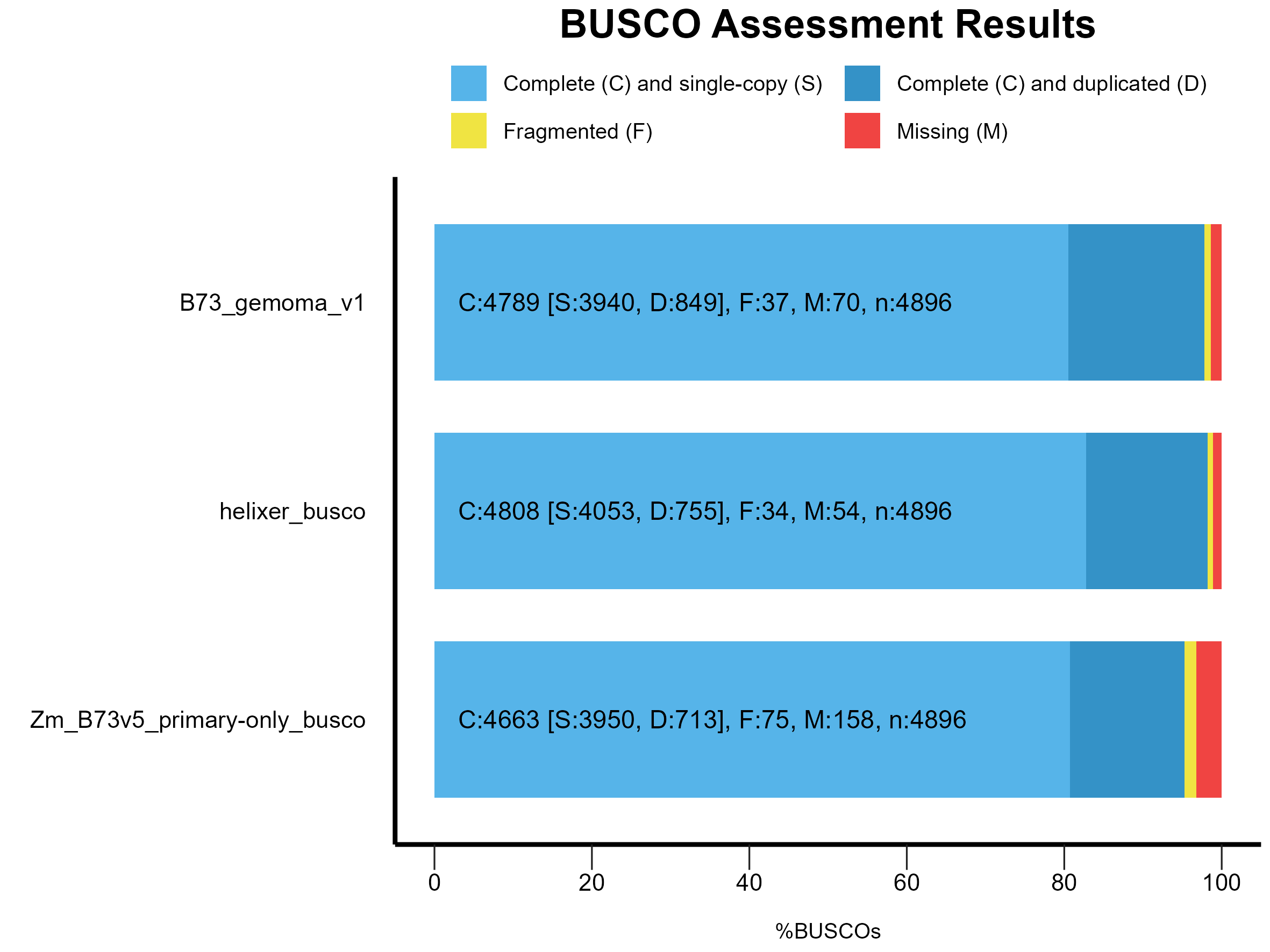
Figure 1: BUSCO results for Helixer, B73.v5 (MaizeGDB) and merged (GeMoMa) annotations.
B. Comparing annotations
Compare Helixer original predictions with GeMoMa:
Compare B73.v5 (MaizeGDB) predictions with GeMoMa:
D. Functional annotation
The Eukaryotic Non-Model Transcriptome Annotation Pipeline (EnTAP) can be used for functional annotation of the predicted genes.
E. Summary Statistics
You can summarize the results using the agat utility:
F. OMArk proteome assessment
OMArk can be used to assess the quality of the predicted proteome:
G. CDS assessments
The plots were generated using the following R script: cds_assesment.R
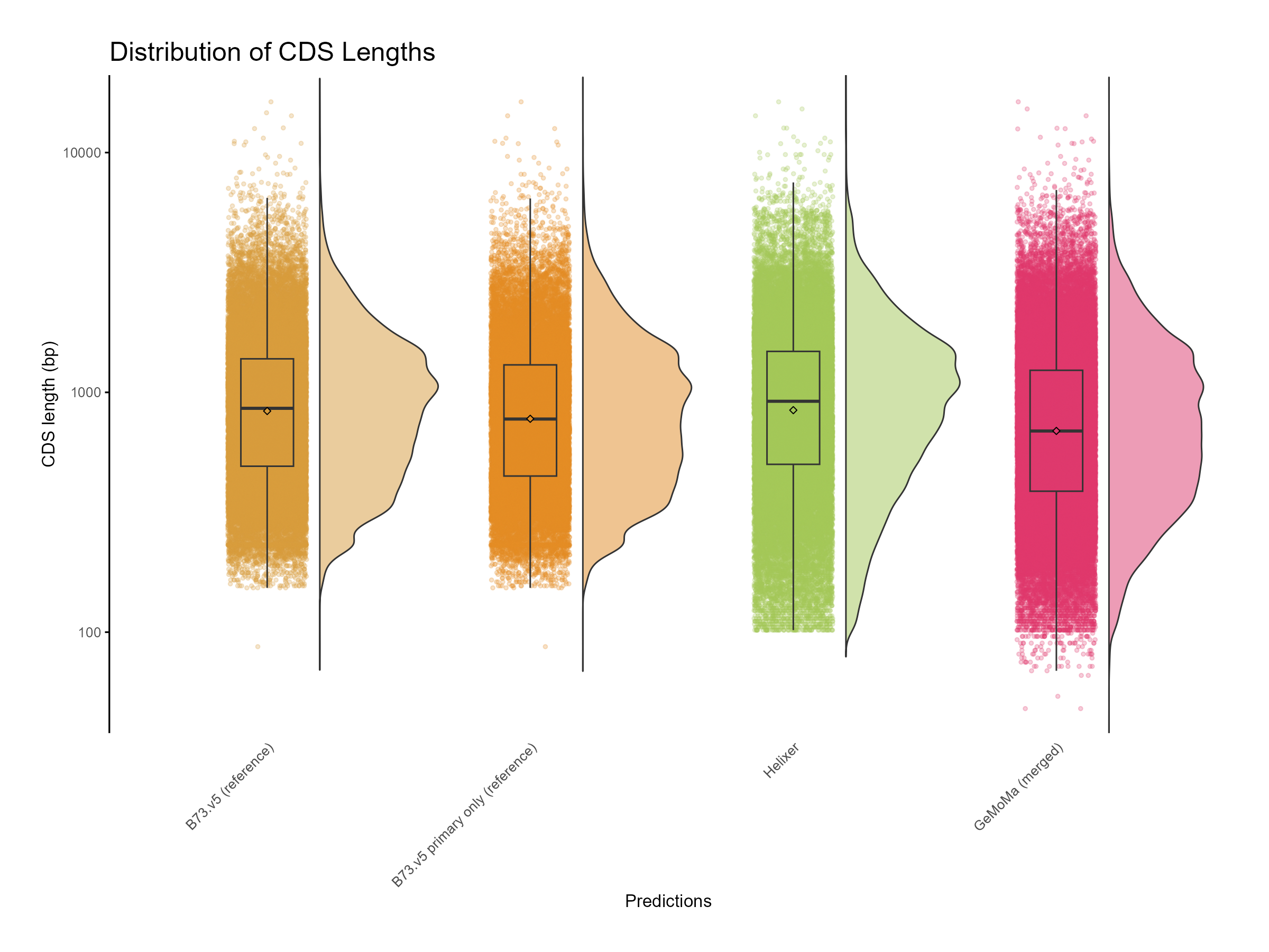
Figure 8: Distribution of CDS length for GeMoMa, Helixer and NAM.v5 predictions.
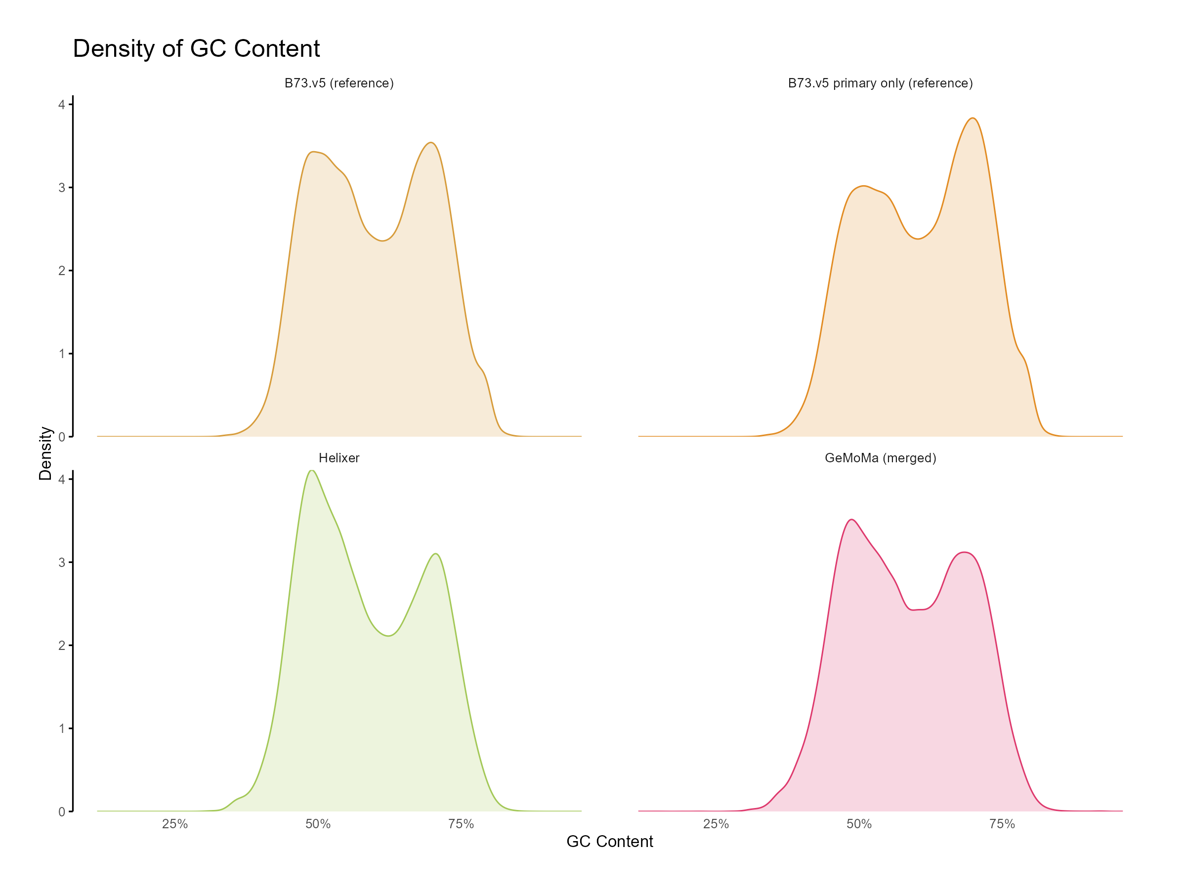
Figure 9: Distribution of GC content for GeMoMa, Helixer and NAM.v5 predictions.
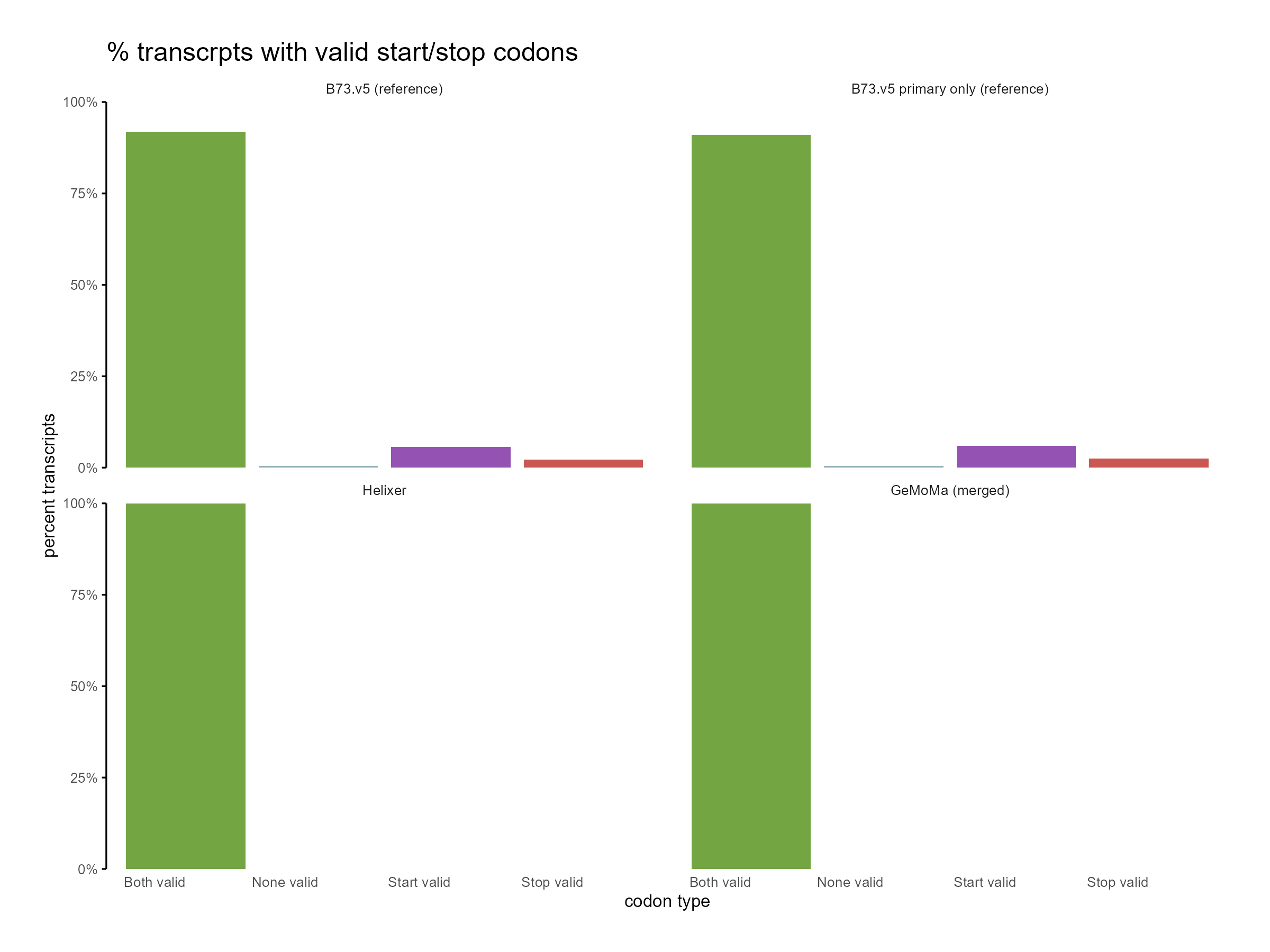
Figure 10: Distribution of start and stop codons for GeMoMa, Helixer and NAM.v5 predictions.