Gene prediction using BRAKER3
BRAKER3 is a pipeline that combines GeneMark-ET and AUGUSTUS to predict genes in eukaryotic genomes. This pipeline is particularly useful for annotating newly sequenced genomes. The flexibility of BRAKER3 allows users to provide various input datasets for improving gene prediction accuracy. In this example, we will use various scenarios to predict genes in a Maize genome using BRAKER3. Following are the scenarios we will cover:
| Input Type | Case 1 | Case 2 | Case 3 | Case 4 | Case 5 | Case 6 | Case 7 | Case 8 |
|---|---|---|---|---|---|---|---|---|
| Genome | ✔️ | ✔️ | ✔️ | ✔️ | ✔️ | ✔️ | ✔️ | ✔️ |
| RNA-Seq | ❌ | ✔️^* | ✔️ | ❌ | ✔️ | ❌ | ❌ | ✔️ |
| Iso-Seq | ❌ | ❌ | ❌ | ❌ | ❌ | ❌ | ✔️ | ✔️ |
| Conserved proteins | ❌ | ❌ | ❌ | ✔️ | ✔️ | ❌ | ✔️ | ✔️ |
| Pretrained species model | ❌ | ❌ | ❌ | ❌ | ❌ | ✔️ | ❌ | ❌ |
minimal RNA-Seq data (one library/one tissue)
Installation
We will use the apptainer tool to build a Singularity container for BRAKER3. The Singularity container will contain all the necessary dependencies and tools required to run BRAKER3. To build the Singularity container, run the following command:
This will create a Singularity container named braker3.sif with BRAKER3 installed.
Setting up BRAKER3
Before running BRAKER3, we need to set up:
GeneMark-ES/ET/EP/ETPlicense key- The
AUGUSTUS_CONFIG_PATHconfiguration path
The license key for GeneMark-ES/ET/EP/ETP can be obtained from the GeneMark website. Once downloaded, you need to place it in your home directory:
For the AUGUSTUS_CONFIG_PATH, we need to copy the config directory from the Singularity container to the scratch directory. This is required because BRAKER3 needs to write to the config directory, and the Singularity container is read-only. To copy the config directory, run the following command:
Running BRAKER3
The paths to the following variables need to be set:
Input datasets
With genome only (no external evidence)
| Input | Type |
|---|---|
| Genome | B73.v5 (softmasked) |
| RNA-Seq data | None |
| Protein sequences | None |
| Long-read data | None |
| Pretrained species model | None |
with minimal RNA-Seq data (one library/one tissue)
| Input | Type |
|---|---|
| Genome | B73.v5 (softmasked) |
| RNA-Seq data | RNAseq (single library) |
| Protein sequences | None |
| Long-read data | None |
| Pretrained species model | None |
with exhaustive RNA-Seq data (11 tissues)
| Input | Type |
|---|---|
| Genome | B73.v5 (softmasked) |
| RNA-Seq data | RNAseq (11 tissues) |
| Protein sequences | None |
| Long-read data | None |
| Pretrained species model | None |
with conserved protein sequences
| Input | Type |
|---|---|
| Genome | B73.v5 (softmasked) |
| RNA-Seq data | None |
| Protein sequences | Viridiplantae protein sequences |
| Long-read data | None |
| Pretrained species model | None |
Using the orthodb-clades tool, we can download protein sequences for a specific clade. In this scenario, since we are using the Maize genome, we can download the clade specific Viridiplantae.fa OrthoDB v12 protein sets.
When this is done, you should see a folder named clade with Viridiplantae.fa in the orthodb-clades directory. We will use this as one of the input datasets for BRAKER3. The following command will run BRAKER3 with the input genome and protein sequences:
with RNA-Seq and conserved protein sequences
| Input | Type |
|---|---|
| Genome | B73.v5 (softmasked) |
| RNA-Seq data | RNAseq (11 tissues) |
| Protein sequences | Viridiplantae protein sequences |
| Long-read data | None |
| Pretrained species model | None |
with pretrained species model ("Maize")
| Input | Type |
|---|---|
| Genome | B73.v5 (softmasked) |
| RNA-Seq data | None |
| Protein sequences | None |
| Long-read data | None |
| Pretrained species model | "Maize" |
with Iso-Seq and conserved protein sequences
| Input | Type |
|---|---|
| Genome | B73.v5 (softmasked) |
| RNA-Seq data | None |
| Protein sequences | Viridiplantae protein sequences |
| Long-read data | Iso-Seq data |
| Pretrained species model | None |
The IsoSeq data for maize (B73) was obtained from the publication PMC7028979 and is available in the ENA BioProject PRJEB32007.
To proceed, you will need the original files listed in the Submitted files: FTP column of the BioProject page. We will download the data (.bam files) and process them using the isoseq3 tool to demultiplex and map the reads to the B73 reference genome.
The primers and adapters required for demultiplexing were sourced from the original publication (Supplementary Table 1).
We will need isoseq_sorted.bam (and merged_B73.fastq) for the case 8 as well.
For this case 7, we only need isoseq_sorted.bam. To setup BRAKER3 with the Iso-Seq data and conserved protein sequences:
with Iso-Seq, RNA-Seq and conserved protein sequences
| Input | Type |
|---|---|
| Genome | B73.v5 (softmasked) |
| RNA-Seq data | RNAseq (11 tissues) |
| Protein sequences | Viridiplantae protein sequences |
| Long-read data | Iso-Seq data |
| Pretrained species model | None |
To run this, you need to first run case 3 (full-RNAseq data) [BRAKER-1] and case 5 (conserved proteins data) [BRAKER-2]. You will also need the Iso-Seq BAM file generated in case 7.
The steps are as follows:
- Run
BRAKERusing the spliced alignments of short-read RNA-seq (here case 3 with full-RNAseq data). - Run
BRAKERusing the conserved proteins data (here case 5 with conserved proteins data). - Run
GeneMarkS-Tprotocol on the Iso-Seq data to predict protein-coding regions in the transcripts:- map the long reads to the genome using minimap2 (here case 7
isoseq_sorted.bam) - collapse redundant isoforms
- predict protein-coding regions using
GeneMarkS-T
- map the long reads to the genome using minimap2 (here case 7
- Run the long read version of
TSEBRAto combine the three gene sets using all extrinsic evidence
Since we have already run case 3 and case 5, we will proceed with the remaining steps.
We will need the hintsfile.gff and augustus.hints.gtf files from case 3 and case 5.
We will also need the gmst.global.gtf file generated from the GeneMarkS-T protocol.
The following command will run TSEBRA to combine the three gene sets:
Processing output
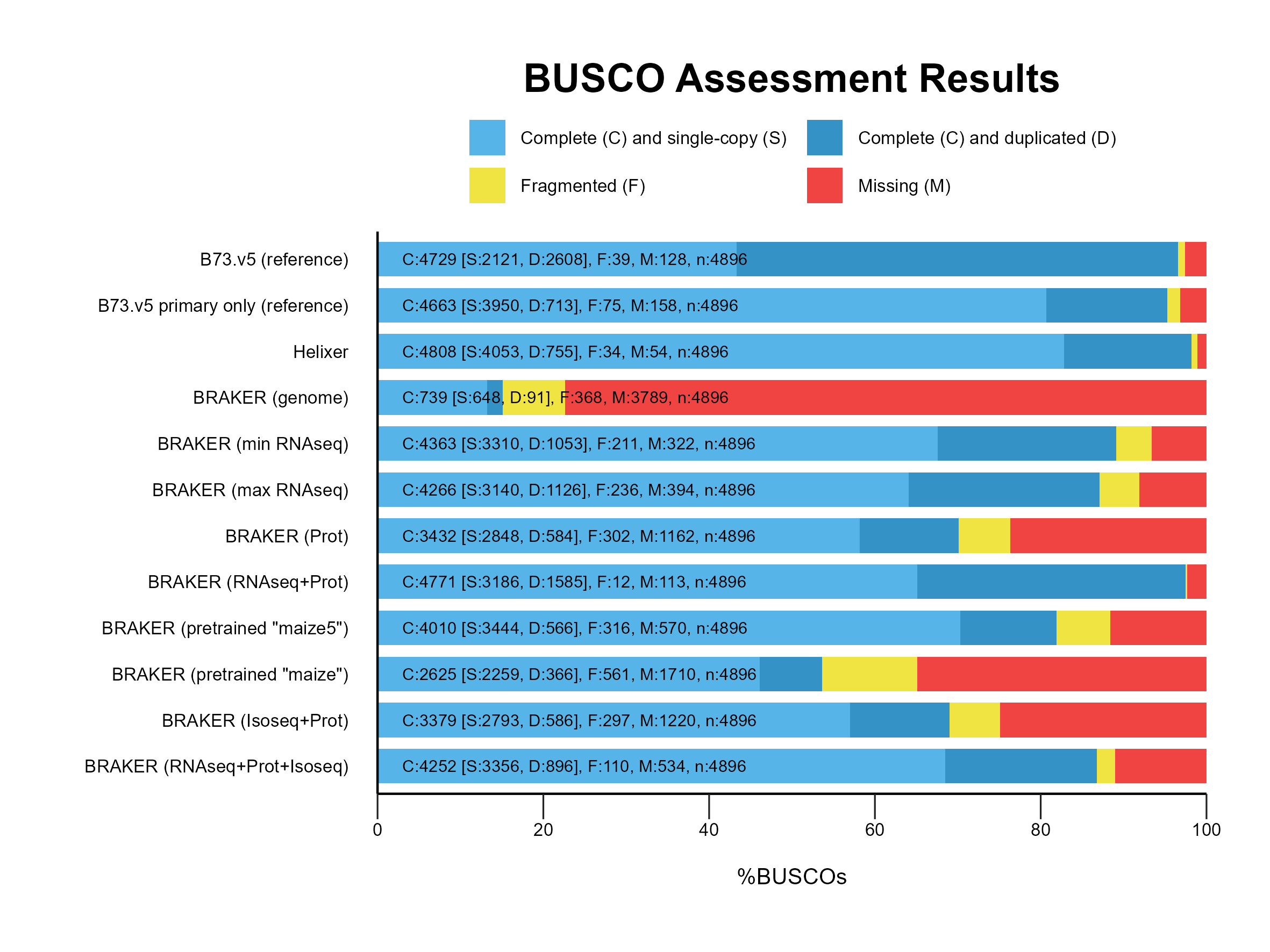
Comparing and Evaluating
A. BUSCO profiling
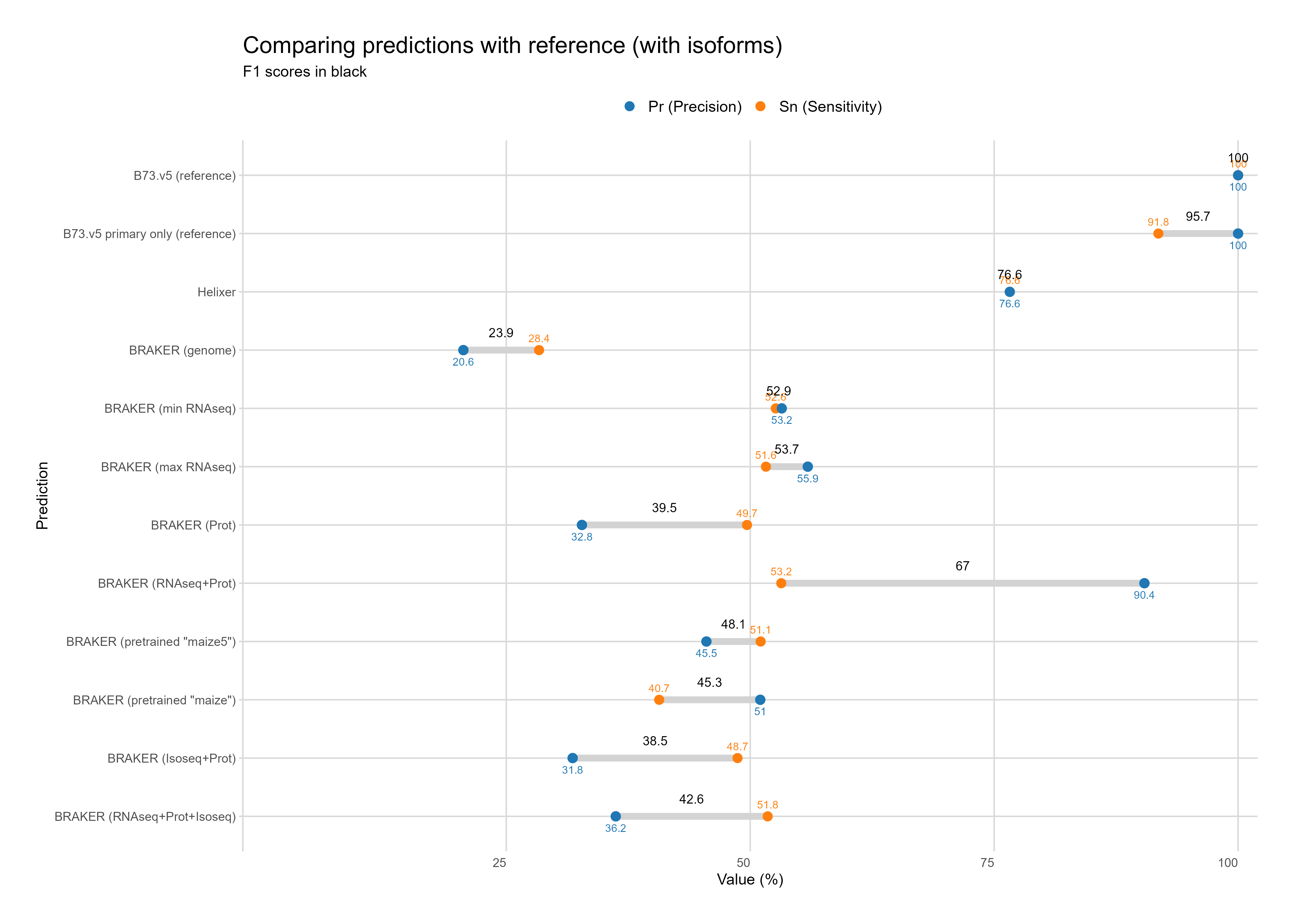
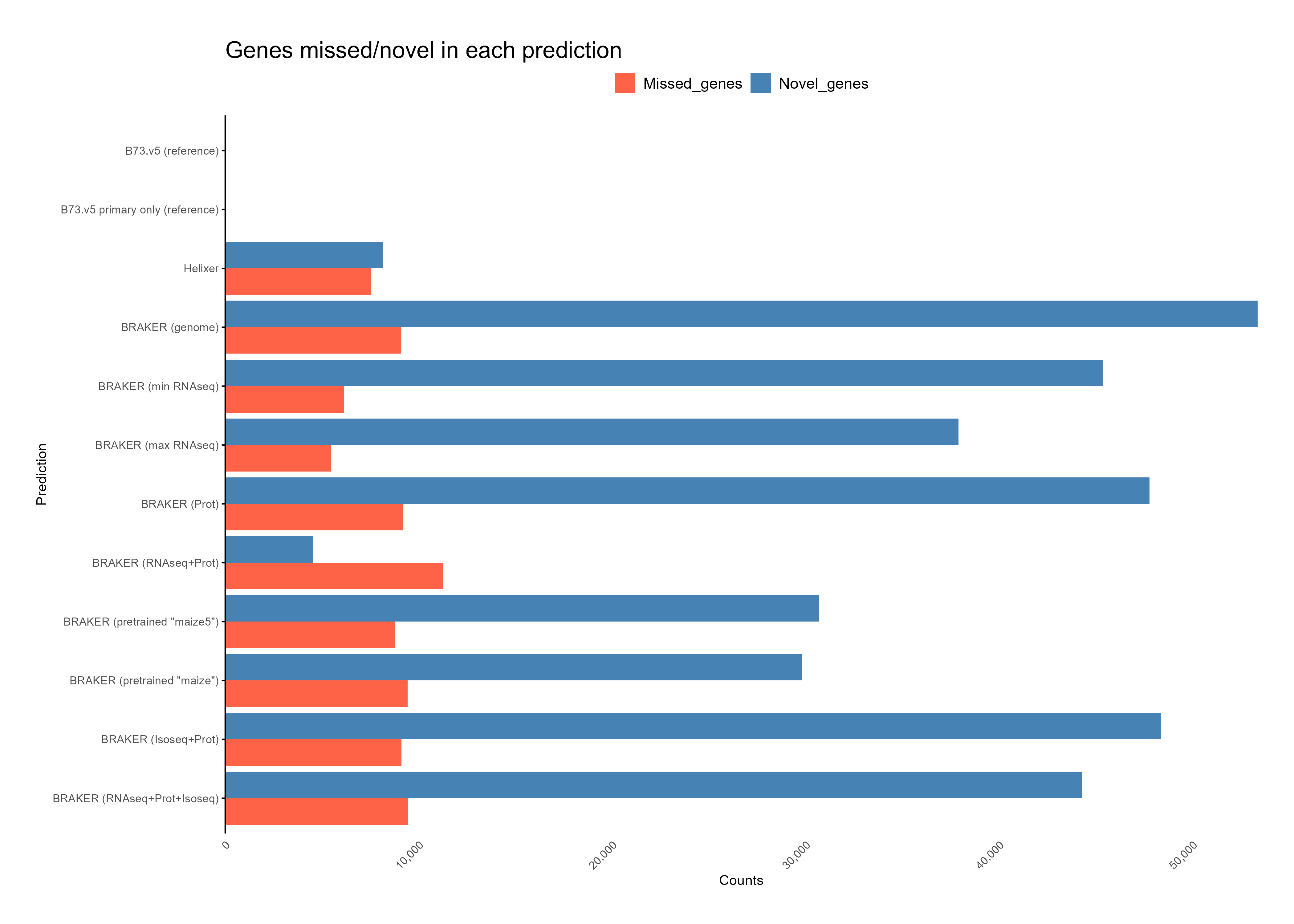
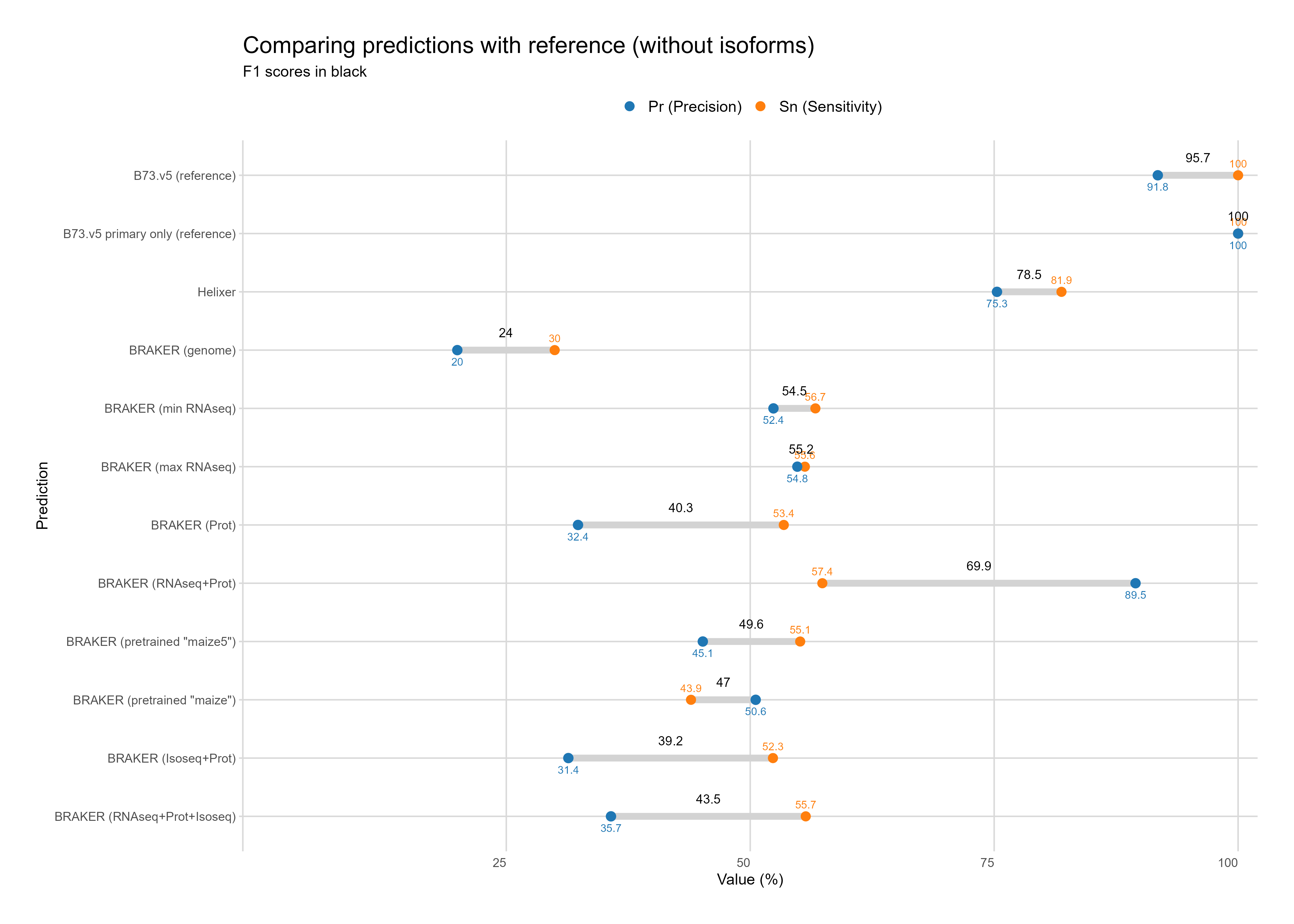
B. Reference comparison
With Isoforms
Without Isoforms

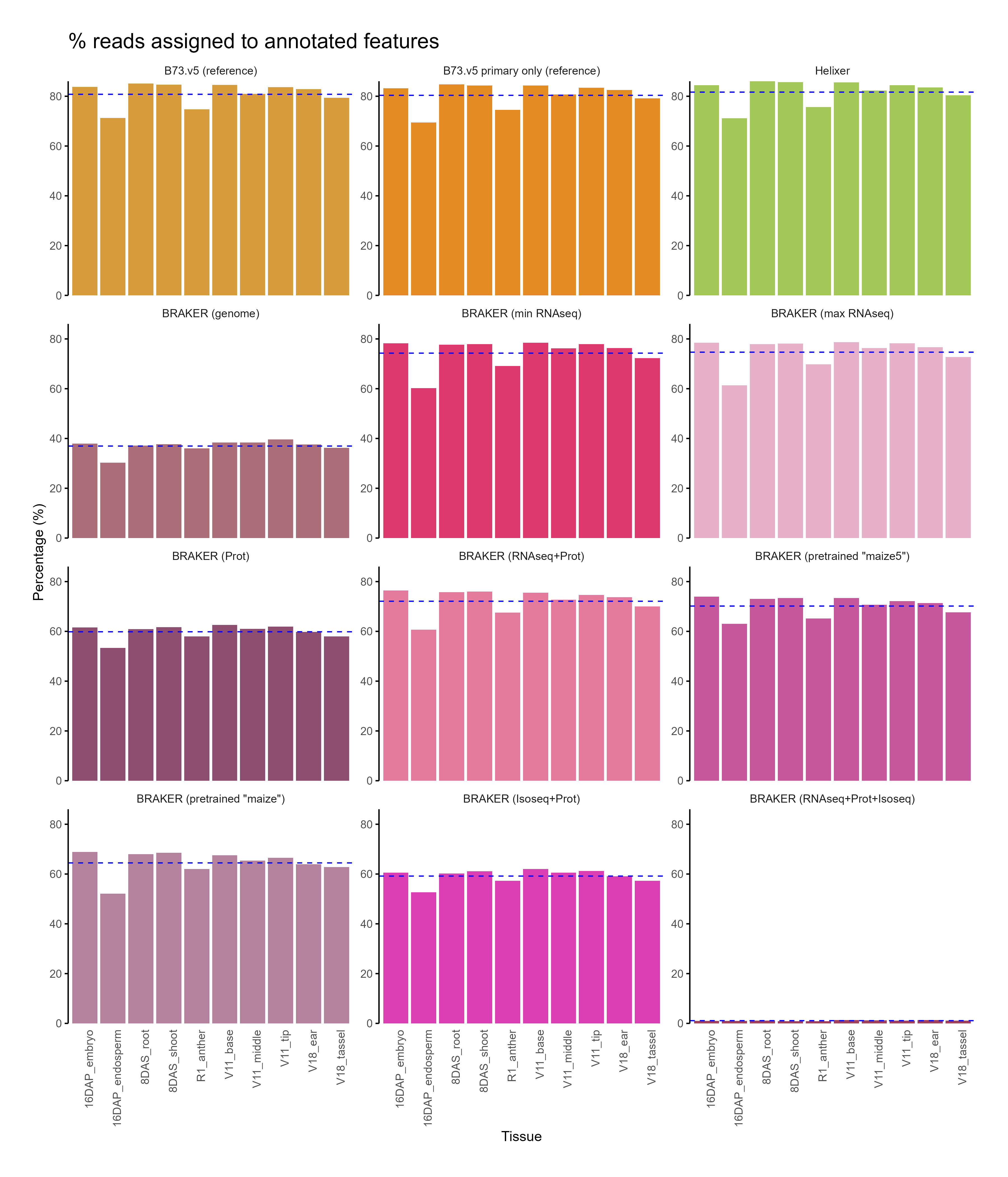
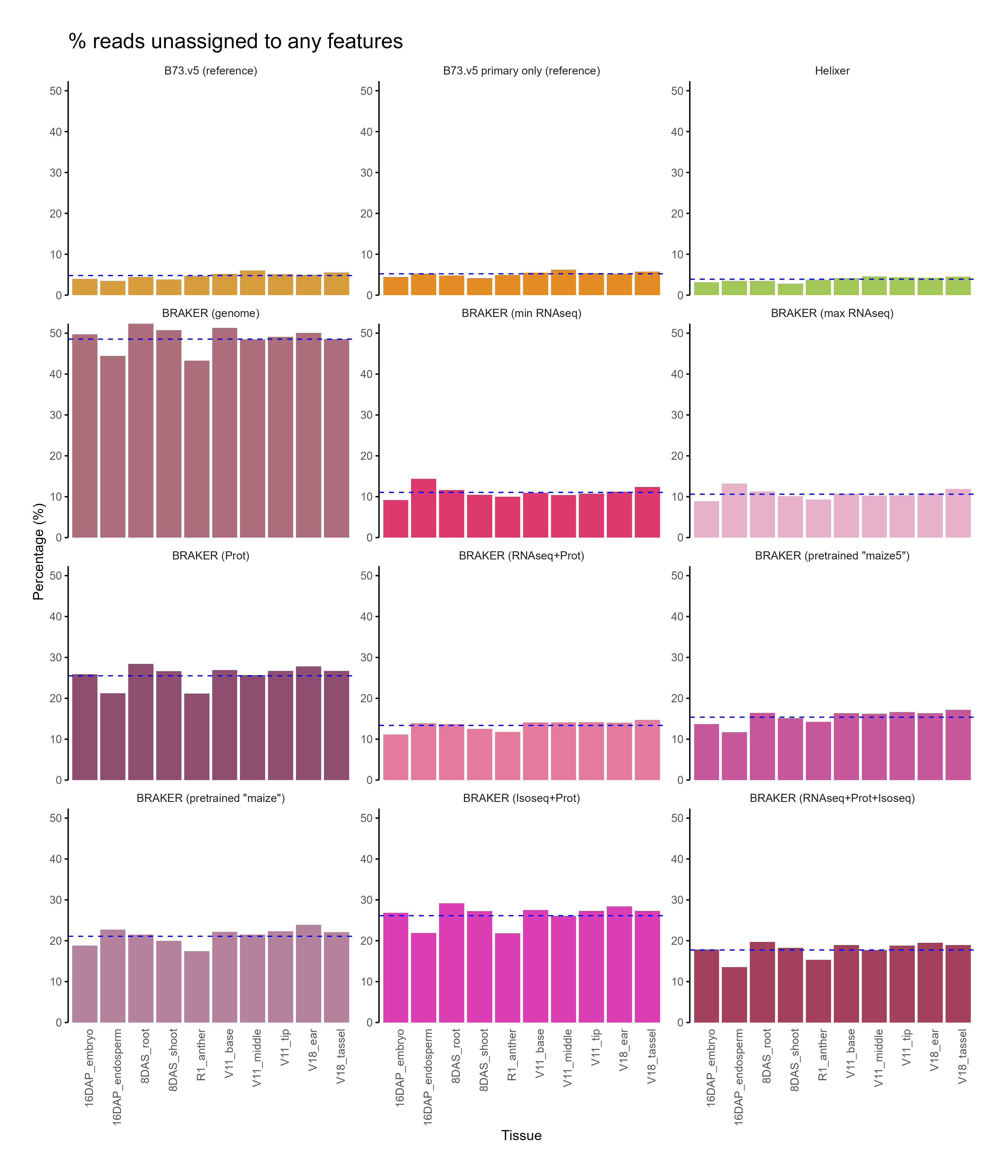
C. Feature assignment
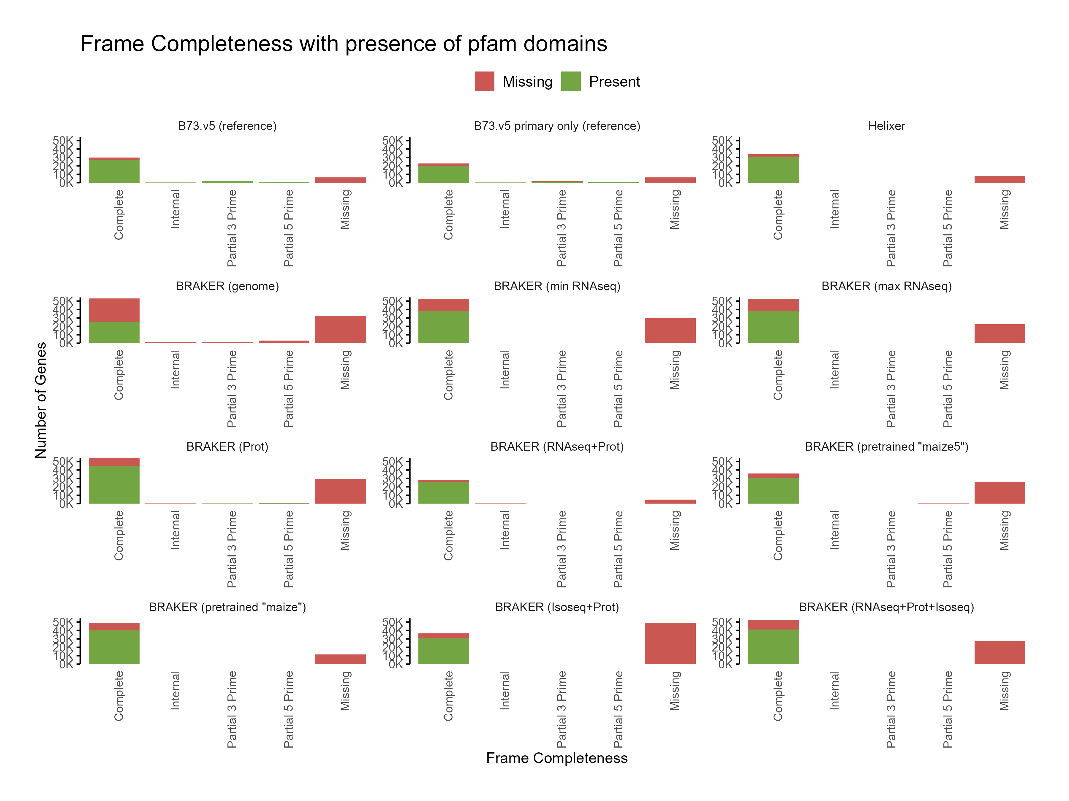
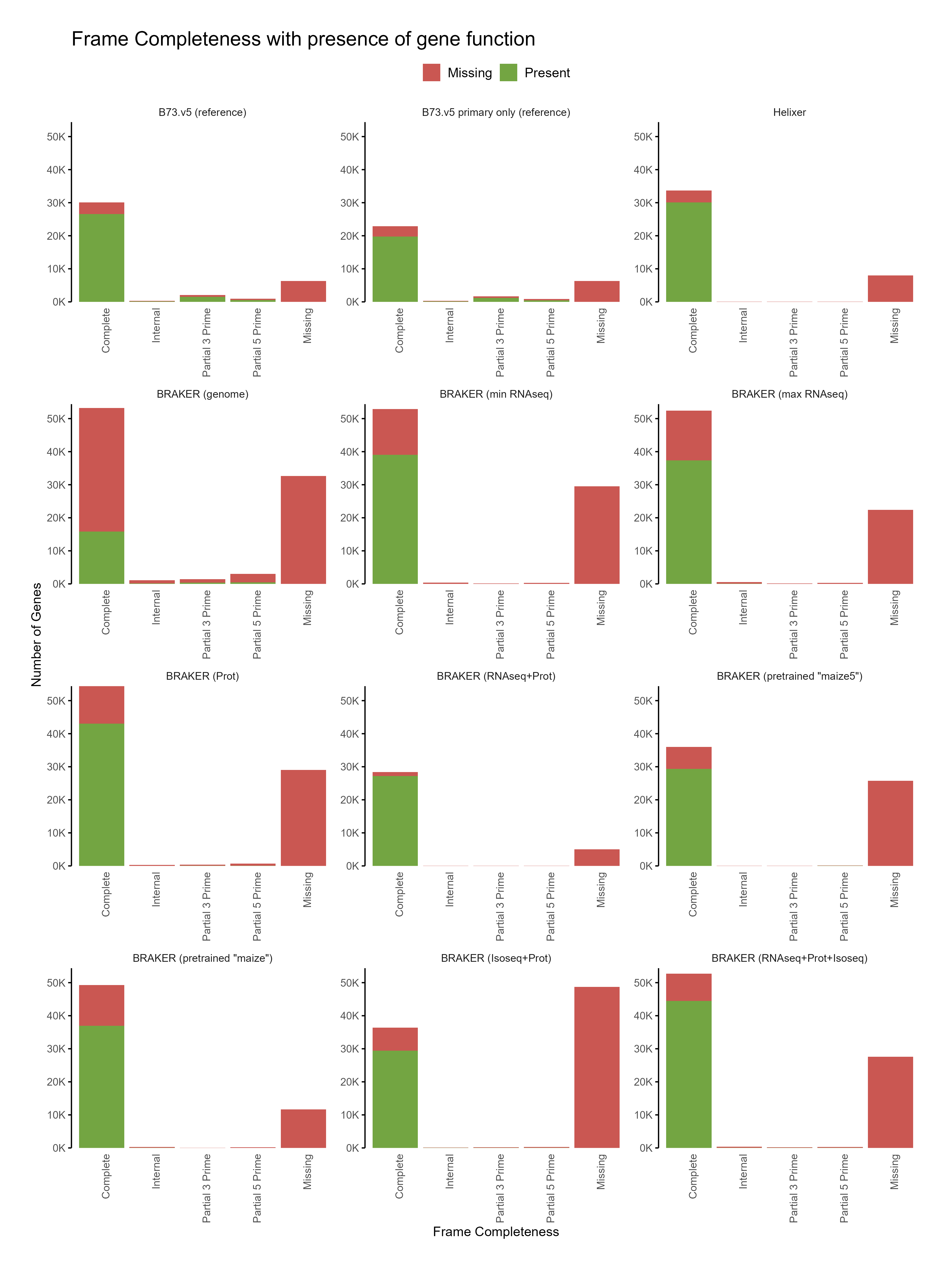
D. Functional annotation
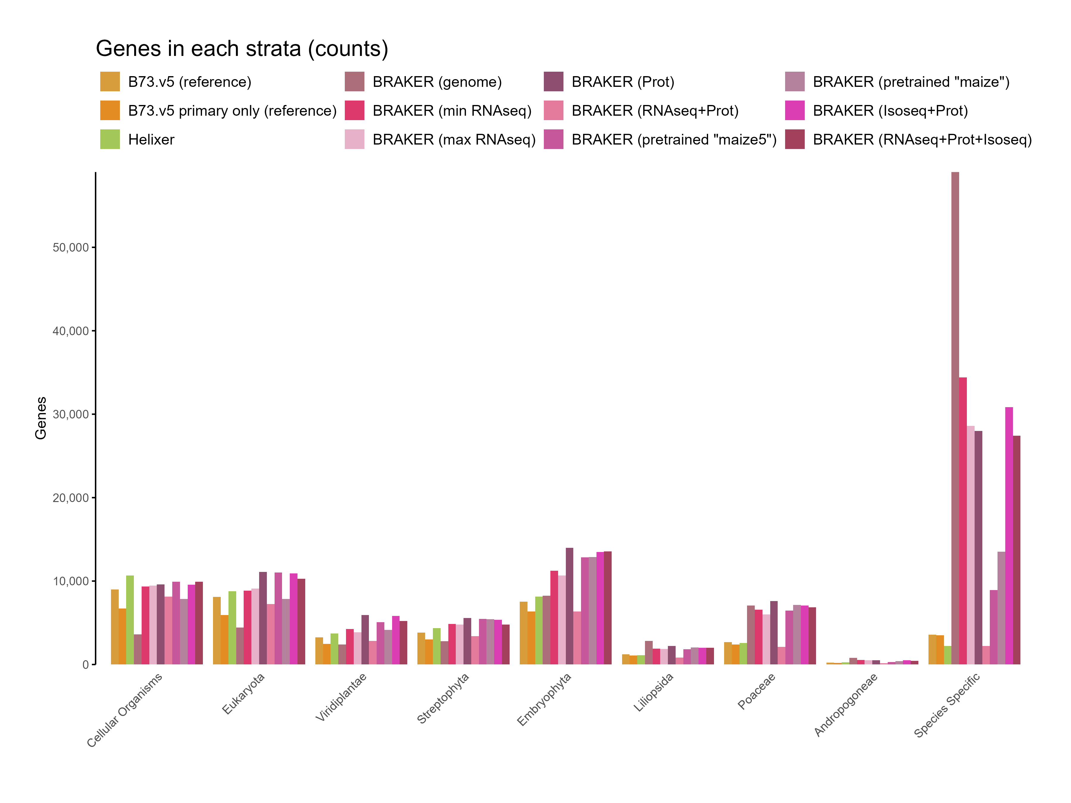
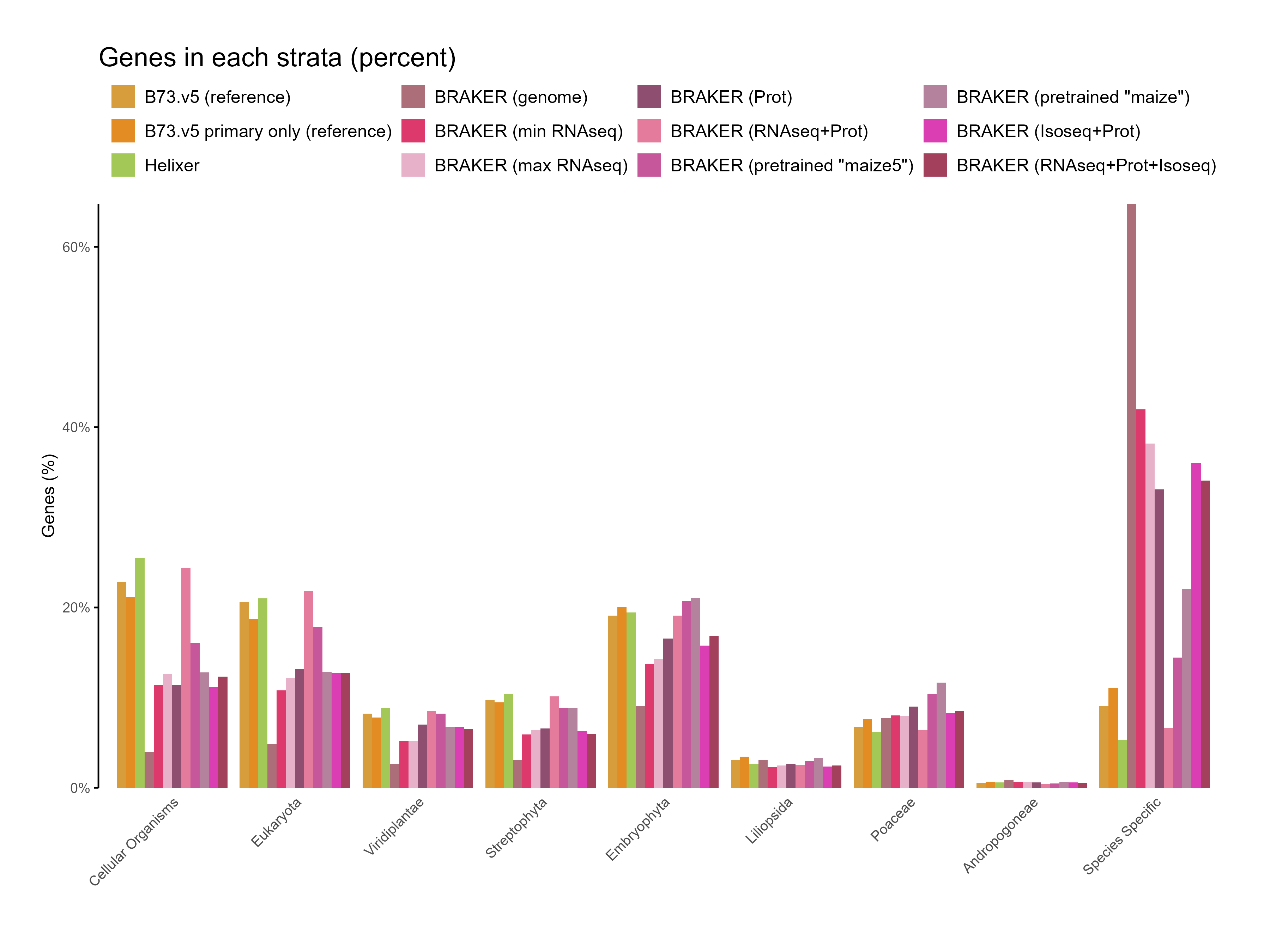
E. Phylostrata analysis
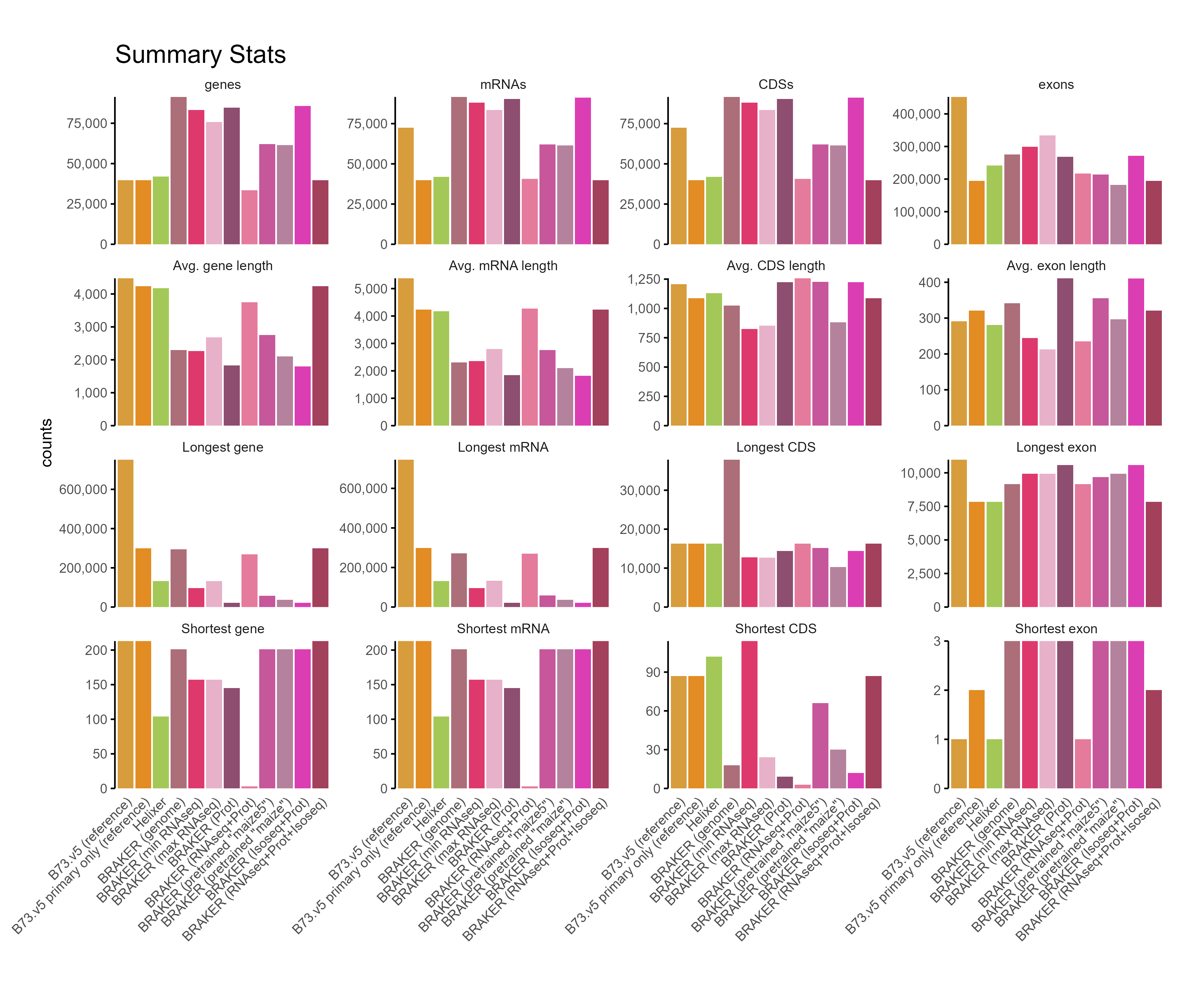
F. GFF3 stats
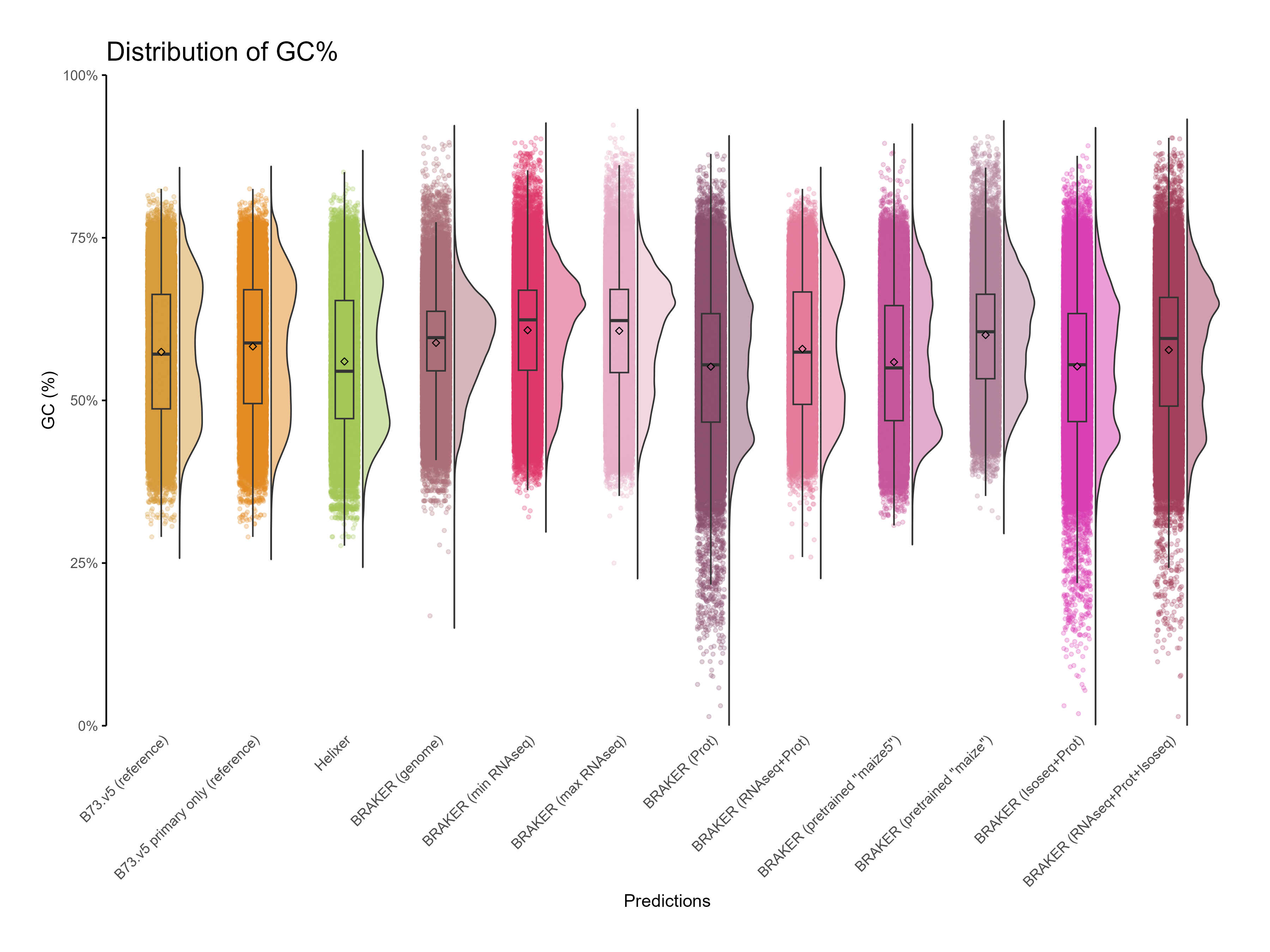
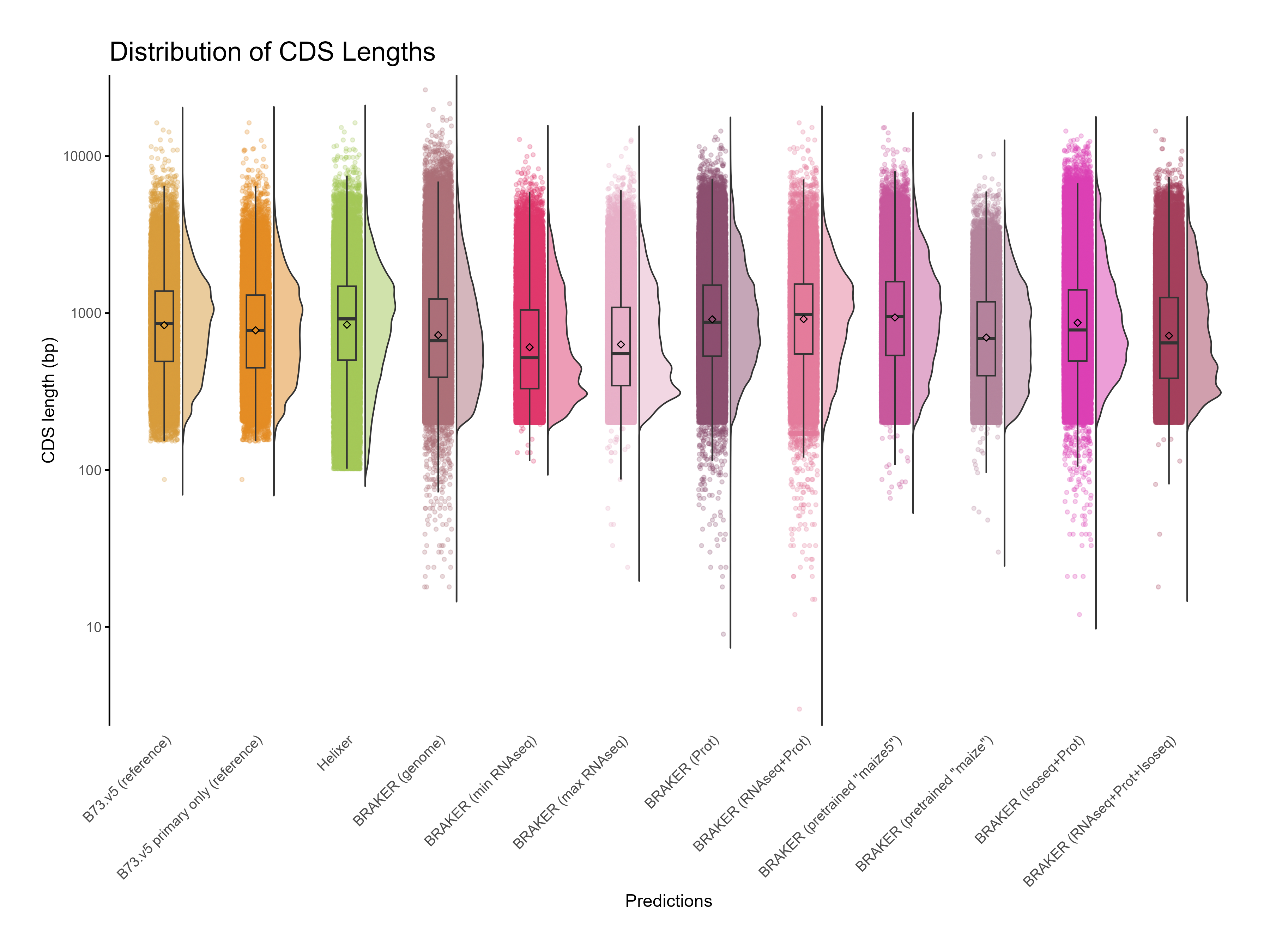
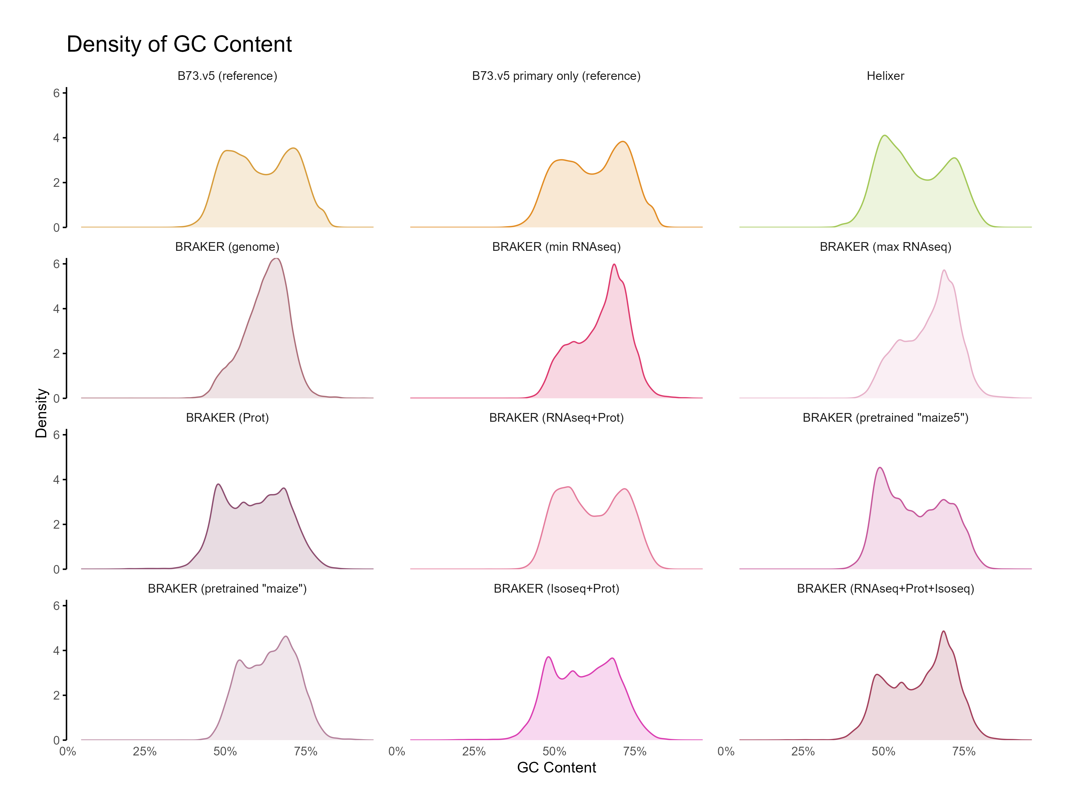
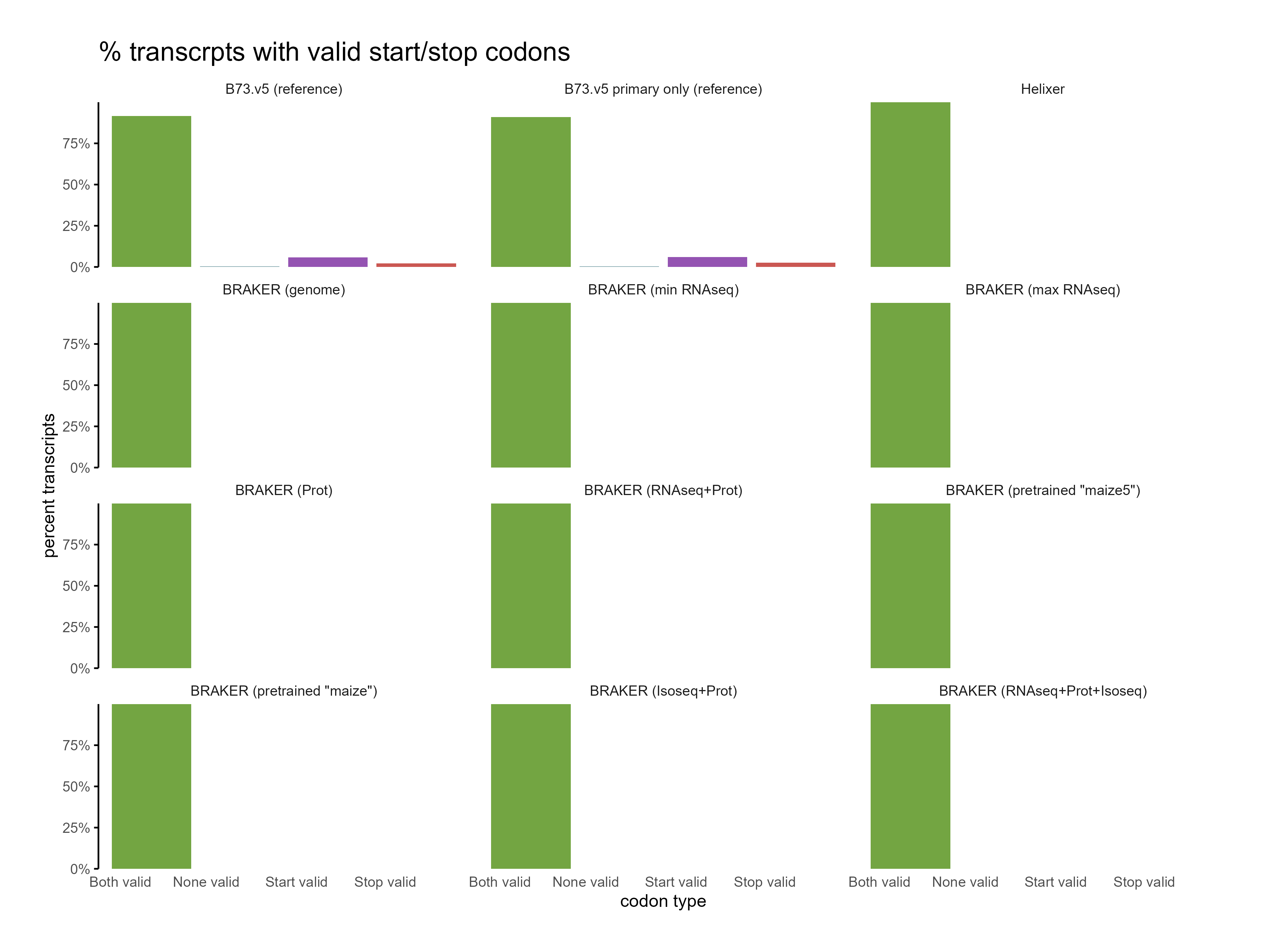
G. OMArk assessment

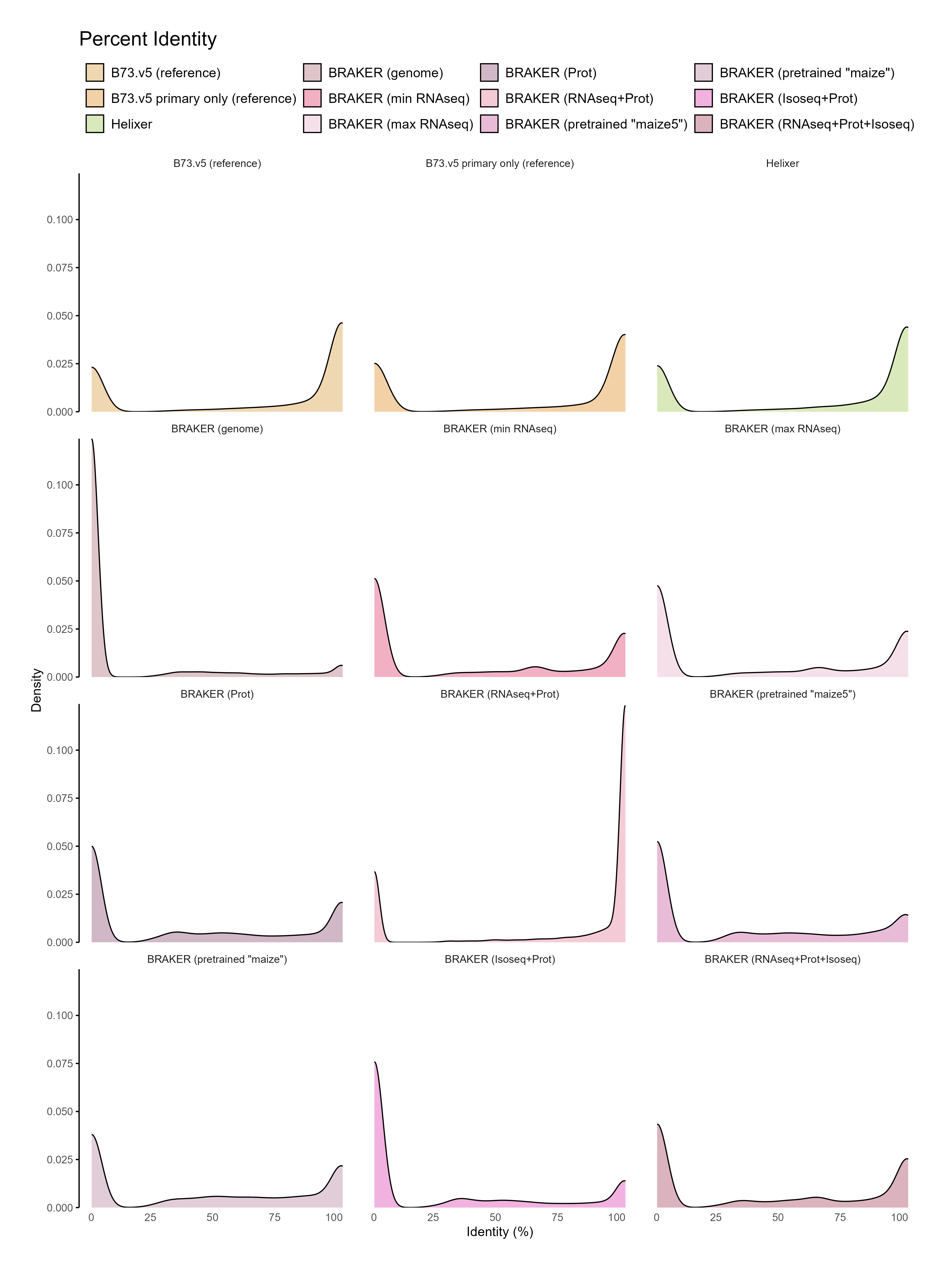
H. CDS assessments